Why AMM Gamma is different from derivatives Gamma

Note: the associated Jupyter notebook is on Github and on Binder.

My last few posts were inspired by the AMM Triangle, and I was discussing the relationship between Divergence Loss (formerly known as Impermanent Loss) and Loss versus Rebalancing. The key thread connecting all of those is the relationship between AMMs, self-financing strategies, and option pricing. In this post I will add another important piece to this puzzle — I will discuss how the Gamma income or bleed is different hedging options versus LPing in an AMM. This may seem only of academic importance, but I am expecting this to have profound implications when looking for optimal fee levels in an AMM. Stay tuned!

Delta hedging and Gamma bleed / gains

It is well known that since Black Scholes Merton’s seminal work from the 1970s onwards that the option pricing formulas they developed are not that much pricing them — this was known at least since Bachelier — but about actually hedging them using the Greek (Delta, Gamma, Theta and friends; see the theammbook.org paper, section 4). BSM’s important insight was that, in a Brownian motion world, options are risk free. Whilst there is a cost replicating them — the Gamma bleed when hedging optionality — but provided volatilities are known, this cost is deterministic.

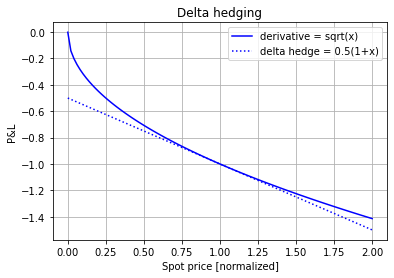
The way options are replicated is through the so-called delta hedge: the option trader runs at every point in time the linear portfolio (ie containing only cash and the risk asset) that best matches the option portfolio. Graphically, this is the well known tangent portfolio in the PV vs spot-price graph below where we see the square-root profile (blue solid line) and its delta hedge (the blue dotted line)

The value of the hedged profile — ie the difference between the profile and its linear approximation — is shown in the blue line below. We also show the quadratic profile that best matches the hedged profile, ie the next term in the Taylor series approximation of it.

The equations for the chart shown above are (ignoring the scaling factors)

Below is the same chart, zoomed in:

Now we are looking what happens when we are delta hedging this profile. We know from Black Scholes Merton that, if we rebalance instantaneously, the replication is perfect. However, what happens when we rebalance less often? We have drawn the expected rebalancing gain (the Gamma gain) against the rebalancing time in the chart below:

First looking at the green dotted line, we see that for the square root profile, the rebalancing time does not matter: as the standard deviation grows in square root t and the gain in x-squared, those two cancel each other out at every horizon. For our actual profile this is not the case, and the reason for this is that the 3rd-order and above terms in the Taylor expansion of the profile become more important.

This is the key reason why the Black Scholes Merton model works so well in practice — markets are not Brownian motions, and rebalancing is not instantaneous, but it does not really matter, as the rebalancing P&L is relatively robust against changes in the rebalancing time because the profile is locally quadratic. So, as long as the rebalancing time is sufficiently short that the quadratic term dominates the Taylor expansion, the effect of Gamma remains relatively stable.

Rebalancing the AMM portfolio

The Gamma in an AMM portfolio is different: it stems from the fact that an AMM this is currently arbitraged to a price x0 trades towards a new price x at the geometric average of x and x0. In our case x0=1, and therefore

which plotted looks like this:

We see that there is a cusp a x=1, rather than the nice quadratic term that appears in derivatives replication

This linear rather than quadratic behaviour around x=1 makes it much steeper for small rebalancing time. In fact, the PV diverges when the rebalancing time goes to zero

For larger rebalancing times of course it crosses over as at this stage the quadratic function outpaces the linear one

Note that the behaviour for small rebalancing times is an extremely important result:

In a perfect Brownian motion world, the value transfer from an AMM to its arbitrageurs diverges, ie it becomes infinite.

This related to the fact that Brownian motion at the microscopic level becomes extremely violent. In other words, the divergence is driven by the small moves: it is well known that a Brownian motion that crosses a given level will cross it an infinite number of times within any open interval containing the touch point (except on a space with measure 0).

However, this is more of a theoretical problem than a practical one: in the real world, there is a maximum frequency at which prices are updated and at which trades happen. This limits the divergence even in a zero-fee environment. In the presence of strictly positive fees, the divergence should disappear even in a Brownian motion environment, because any level of fees strictly greater than zero breaks the divergence at the rebalancing time t=0. Having said this — this also suggests that the profitability of a liquidity position depends non-trivially on the fee levels, but this is subject of future work. In this context I would like to point out the paper by Tassy and White that has some interesting analytics in this respect.