Zero-Copy Sliding Windows: How to Reduce Memory Cost in Quantitative Deep Learning

In quantitative machine learning the bottleneck is almost never the model. It is the data pipeline feeding it. If your pipeline is slow and wasting memory, your GPU will just do nothing until the next batc

When you feed 100 tickers of time-series data through 60-step sliding windows into a PyTorch model the standard approach creates over 41,000 separate NumPy arrays in memory. Forty-one thousand copies of nearly identical data were created before the model trained a single batch.

And this is a tiny dataset. For a serious quant work sometimes you have thousands of tickers, intraday bars, and dozens of engineered features on top of raw prices.

There’s a more efficient method than using naive sliding windows.

In this article I’ll walk you through zero-copy index map architecture that can cut memory peak by 38% and triple your pipeline speed. We will look under the hood of PyTorch, Numpy and Polars, discuss failure modes, examples on optimization and how you can build a production-grade quant engineering pipeline, using Polars and PyTorch.

If in hurry, here’s the repo

The Problem: Why Sliding Windows Explode Your Memory

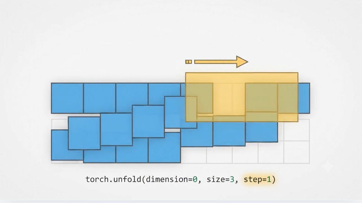
To train a neural network on sequential data, you need to feed it overlapping sliding windows. For example, if you want to predict tomorrow’s stock return, you might give your model the last 60 days of historical features. To build the next training example, you slide the window forward by one day.

Mathematically, if your features are represented by a sequence X, your first training window is X{1:60}. Your second window is X{2:61}. Your third is X{3:62}. Notice the overlap?

Time steps 2 through 60 are repeated in the first and second windows. Time steps 3 through 60 are repeated in the first, second, and third windows. If you physically copy these windows into new memory buffers, you are duplicating the same data over and over again. This duplication is quadratic in the window length.

But, when you are building a serious quant model, you do not train once.

You run hyperparameter searches across window sizes, sequence lengths, feature subsets, and normalization strategies. For example, this recent paper From the Oxford-Man Institute evaluated over a dozen models including LSTMs, Transformers, Mamba, and hybrid VSN architectures across 15 years of daily futures data. The computational bottleneck was not GPU compute time. It was fitting dataset variations into RAM simultaneously to allow parallel evaluation.

If one experiment costs 129 MB of RAM, running 4 in parallel costs 516 MB just for dataset objects.

Add model weights, gradients, optimizer states, and GPU transfer buffers on top, and your memory explodes. So you serialize. One experiment finishes, you clear it from memory, load the next. That’s not efficient. Zero-copy architecture solves this, all experiments point into the same underlying memory blocks.

Below is the standard PyTorch Dataset pattern that most developers write when they first start out. If you’re not familiar with how to construct the Dataset, I recommend reading this article from Sebastian Raschka that will walk you through the most basic concepts you need to know.

class TimeSeriesDataset(Dataset):
    """PyTorch Dataset that produces sliding windows from grouped time-series data
       This version is NOT optimized"""
    def __init__(
        self, 
        df,
        feature_cols,
        target_cols,
        sequence_len,
        group_col : str = "ticker",
        date_col: str = "date",
    ):
        self.sequence_len = sequence_len
        self.feature_cols = feature_cols
        self.target_cols = target_cols

        self._windows: list[tuple[np.ndarray, np.ndarray]] = []

        df = df.sort(group_col, date_col)

        for group_name, group_df in df.group_by(group_col, maintain_order=True):
            n_rows = group_df.height
            ticker_name = group_name[0] if isinstance(group_name, tuple) else group_name
            if n_rows < sequence_len + 1:   
                continue

            features_np = group_df.select(feature_cols).to_numpy().astype(np.float32)
            targets_np = group_df.select(target_cols).to_numpy().astype(np.float32)

            for i in range(n_rows - sequence_len):
                feature_window = features_np[i:i+sequence_len]
                target_vector = targets_np[i+sequence_len-1]
                self._windows.append((feature_window, target_vector))

    def __len__(self):
        return len(self._windows)

    def __getitem__(self, idx):
        features, targets = self._windows[idx]
        return (
            torch.from_numpy(features),
            torch.from_numpy(targets),
        )

Don’t panic, we’re interested in this loop that starts at this line: for i in range(n_rows - sequence_len). It generates the start offsets for every valid sliding window inside a ticker's dataset and ensures every sample has the exact number of historical steps required by your model. The result: 41,000 slices.

Why does this fail?

Even though NumPy slicing creates views instead of copies, we still get memory hog because storing 41,000 slices in a Python list means managing 41,000 separate NumPy array objects and 41,000 tuple objects. This adds up to tens of megabytes of pure metadata.

And when you send data from the dataset to the PyTorch workers, Python must serialize each item. When it serializes a NumPy slice view, it cannot easily serialize just the view. Instead, it serializes the underlying base array or copies the slice into a new contiguous memory block. This triggers massive memory copying.

As a result, if you scale this to intraday data, your machine will run out of memory before the training loop even starts.

The Solution: Zero-Copy Index Map

To solve this, we must separate the raw data from the window coordinates. Instead of slicing arrays and storing those slices during initialization, we store the raw data as large, contiguous blocks of memory (one block per ticker). Then, we create a map to keep track of where the windows start.

self._feature_blocks: list[torch.Tensor] = []
self._target_blocks: list[torch.Tensor] = []
self._index_map: list[tuple[int, int]] = []

Instead of holding thousands of tiny arrays, the first two lists will hold exactly N tensors, where N is the number of tickers in your dataset (in our case, 100). And the third list will hold coordinate pairs — block id and start.

The block_idx tells us which ticker's tensor to look at, and the start integer tells us the row index where our window begins. Because these are standard Python integers, each tuple requires only 56 bytes. A 60-step window of 60 features requires 14,400 bytes. The coordinate tuple is 257 times smaller than the actual data.

block_idx = len(self._feature_blocks)
self._feature_blocks.append(torch.from_numpy(features_np))
self._target_blocks.append(torch.from_numpy(targets_np))
n_windows = n_rows - sequence_len

for i in range(n_windows):
 self._index_map.append((block_idx, i))

PyTorch does not have a native method to import or read Polars DataFrame objects directly, that’s why we convert to numpy first and once the data is in this contiguous numpy format, calling torch.from_numpy() is a zero-copy operation.

Continue reading at https://zaurtarunov.substack.com.

P.S. I’m building an open sourced ML repository for quant finance where you can learn and optimize your models and strategies. Give it a star. If you wish to contribute, feel free to fork and get in touch!