Optuna optimization history and hyperparameter importance charts.

Why define-by-run search spaces, adaptive sampling, and pruning make model tuning faster, cheaper, and far more practical than exhaustive search.

Introduction

If you have ever launched a GridSearchCV on Friday afternoon and hoped Monday would bring clarity, you already know the pattern. Hours or days later, you get a best configuration, a modest lift in validation score, and the uncomfortable feeling that most of the runs taught you almost nothing.

Hyperparameter tuning matters. In many projects, the difference between a model that is merely acceptable and one that is genuinely deployable does not come from inventing a brand new architecture. It comes from getting the training recipe right: the learning rate, the regularization strength, the tree depth, the number of estimators, the optimizer, the batch size, the scheduler, and all the other knobs that shape how the model actually learns.

The problem is that the default answer many teams still reach for, grid search, treats the search space as if every region deserves the same attention. Real models do not behave that way.

This is where Optuna earns its place.

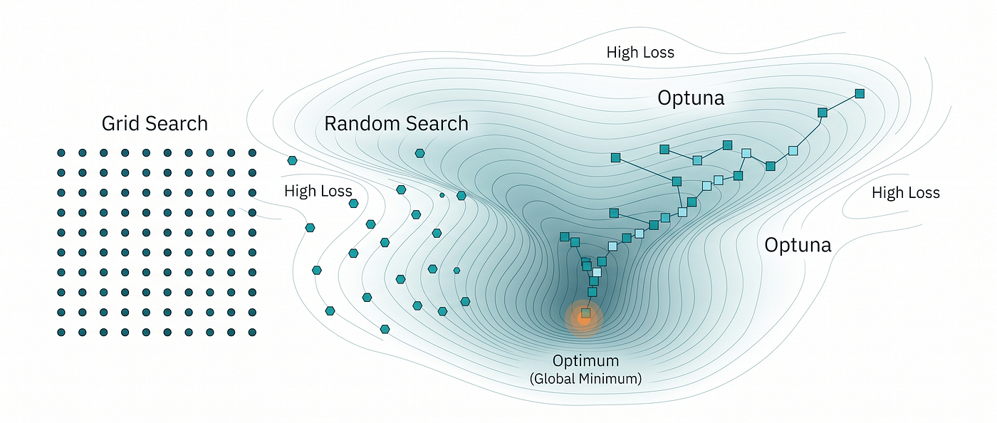
Optuna is often described as a library for “optimizing grid search,” but that is not really the right mental model. Grid search is the brute-force baseline that Optuna helps you move beyond. Optuna is better understood as a general purpose hyperparameter optimization framework: it learns from previous trials, concentrates future trials in more promising regions of the space, and can stop weak candidates early before they consume the full training budget.

In practice, that means fewer wasted experiments, faster iteration cycles, and a much more realistic way to tune modern machine learning systems.

In this article, we will look at why grid search becomes wasteful, how Optuna works, what “define-by-run” means in practice, and how to build a useful Optuna workflow with scikit-learn. We will also cover pruning, visualization, and the scenarios where Optuna is the right tool, and where it is not.

Why grid search becomes wasteful

Grid search has one major advantage: it is easy to explain. You choose a discrete set of values for each hyperparameter, evaluate every combination, and keep the best one.

The problem is that this simplicity collapses as soon as the search space becomes even moderately realistic.

Suppose you want to tune five hyperparameters and assign ten candidate values to each. That is already:

10 x 10 x 10 x 10 x 10 = 100,000 combinations

Even if a single run only takes two minutes, the full search would require almost 139 days of compute if executed sequentially.

But the compute cost is only part of the problem. Grid search also assumes uniform importance across the search space. In reality, some hyperparameters matter far more than others. Some matter only in interaction with specific settings. Some should be searched on a logarithmic scale rather than linearly. A learning rate of 0.001, 0.01, and 0.1 is often far more informative than 0.01, 0.02, and 0.03, yet a naive grid does not encode that intuition naturally.

This is why random search often beats grid search as a baseline: with the same budget, it explores more distinct regions. And this is also why adaptive optimization frameworks such as Optuna are useful: they do not just sample broadly, they sample with feedback.

The practical difference is simple:

> Grid search asks, “What if we try everything?” Optuna asks, “What should we try next?”

A fixed grid spends budget everywhere, even where it is very unlikely to help.

What Optuna actually is

At a high level, Optuna revolves around a few core concepts:

• Study: the full optimization process.

• Trial: one execution of the objective function.

• Objective: the function that trains and evaluates your model.

• Sampler: the algorithm that decides which hyperparameters to try next.

• Pruner: the mechanism that stops unpromising trials early.

That vocabulary matters because it reflects how Optuna thinks about optimization. You are not handing it a rigid parameter grid. You are defining an objective function, and Optuna repeatedly executes it under different parameter choices.

The default sampler is TPESampler, based on the Tree structured Parzen Estimator algorithm. Without going too deep into the mathematics, the key idea is straightforward: Optuna separates past trials into better and worse groups, estimates where good trials tend to live, and biases future sampling toward those regions. In other words, it allocates search budget where the evidence says it is most likely to pay off.

This is already a major step beyond exhaustive search.

On top of that, Optuna supports persistent storage, parallel execution, dashboard based monitoring, and visualization functions that make the optimization process inspectable rather than opaque. That makes it useful not only for experimentation, but also for repeatable team workflows.

The design choice that makes Optuna feel natural: define-by-run

One of Optuna’s most important ideas is its define-by-run API.

Instead of declaring the whole search space in a separate configuration object, you define it directly inside Python code, in the same place where the training logic lives. That means the search space can depend on conditionals, loops, feature flags, or model families.

For example:

def objective(trial):
    model_name = trial.suggest_categorical("model", ["random_forest", "svm"])

    if model_name == "random_forest":
        max_depth = trial.suggest_int("rf_max_depth", 3, 20)
        min_samples_split = trial.suggest_int("rf_min_samples_split", 2, 20)

        # train RandomForest here

    else:
        c_value = trial.suggest_float("svm_c", 1e-3, 1e3, log=True)
        kernel = trial.suggest_categorical("svm_kernel", ["linear", "rbf"])

        # train SVM her

Define-by-run in practice: the search space is built dynamically based on the model selected in each trial.

This looks like normal Python because it is normal Python.

That may sound like a small ergonomic detail, but it solves a very real limitation of many older tuning frameworks. Real model pipelines are not flat tables of independent parameters. They are conditional systems: parameters exist only when a certain model is selected, a specific optimizer is enabled, or a certain preprocessing branch is active. Optuna handles this naturally because the search space is created dynamically during execution.

This is one of the main reasons it integrates so well with practical ML code.

Optuna’s define-by-run approach makes conditional search spaces feel like ordinary Python.

The mental shift from param_grid to objective

For teams coming from scikit-learn’s GridSearchCV, the hardest part of adopting Optuna is usually not technical. It is conceptual.

With grid search, you describe a list of candidate values:

param_grid = {
"max_depth": [3, 5, 7, 9],
"min_samples_split": [2, 5, 10],
}

Classic grid representation: candidate values are declared up front for every hyperparameter.

With Optuna, you describe how a trial should generate values:

def objective(trial):
    max_depth = trial.suggest_int("max_depth", 3, 9)
    min_samples_split = trial.suggest_int("min_samples_split", 2, 10)

Optuna version of the same idea: instead of enumerating all combinations, each trial samples values within defined ranges.

That shift matters because it gives you a different kind of control. You are no longer enumerating everything up front. You are defining a search process. This is what makes conditional parameters, logarithmic ranges, and adaptive exploration feel natural instead of awkward.

Once you internalize that change, Optuna stops feeling like a specialized optimization library and starts feeling like a clean extension of ordinary Python experimentation.

A first Optuna study in practice

Let us start with a compact but realistic example using scikit-learn. We will tune a RandomForestClassifier on the breast cancer dataset using cross-validated ROC AUC.

import optuna

from sklearn.datasets import load_breast_cancer
from sklearn.ensemble import RandomForestClassifier
from sklearn.model_selection import StratifiedKFold, cross_val_score

X, y = load_breast_cancer(return_X_y=True)

cv = StratifiedKFold(
    n_splits=5,
    shuffle=True,
    random_state=42
)

def objective(trial: optuna.Trial) -> float:
    params = {
        "n_estimators": trial.suggest_int("n_estimators", 100, 600),
        "max_depth": trial.suggest_int("max_depth", 3, 20),
        "min_samples_split": trial.suggest_int("min_samples_split", 2, 20),
        "min_samples_leaf": trial.suggest_int("min_samples_leaf", 1, 10),

        "max_features": trial.suggest_categorical(
            "max_features",
            ["sqrt", "log2", None]
        ),

        "class_weight": trial.suggest_categorical(
            "class_weight",
            [None, "balanced"]
        ),

        "random_state": 42,
        "n_jobs": 1,
    }

    model = RandomForestClassifier(**params)

    score = cross_val_score(
        model,
        X,
        y,
        cv=cv,
        scoring="roc_auc",
        n_jobs=-1,
    ).mean()

    return score

study = optuna.create_study(
    direction="maximize",
    study_name="rf_breast_cancer",
    storage="sqlite:///optuna_demo.db",
    load_if_exists=True,
)

study.optimize(objective, n_trials=50)

print("Best ROC AUC:", study.best_value)
print("Best params:", study.best_params)

First end to end Optuna + scikit-learn workflow: objective definition, cross validated evaluation, and SQLite-backed study persistence.

There are a few reasons this example is more realistic than many toy optimization demos.

First, the search space is not arbitrary. It encodes domain knowledge. We are not testing n_estimators from 1 to 5000, because that would mostly waste time. We are also using categorical choices where the parameter is truly discrete and bounded integer ranges where the effect is monotonic enough to justify it.

Second, the metric is cross-validated ROC AUC, not a single train/validation split. That matters. If the objective itself is noisy, the optimizer will chase randomness rather than signal.

Third, the study uses SQLite storage. This is not mandatory, but it immediately makes the workflow more practical. You can stop and resume the study, inspect the results later, or point Optuna Dashboard at the same database.

One practical implementation detail: in code like this, it is usually better to keep parallelism at one level. Here, cross-validation runs in parallel while each individual Random Forest fit stays single process, which avoids oversubscribing CPU cores.

In many real projects, fifty intelligent trials like this can outperform a much larger exhaustive grid, simply because the budget is being spent more selectively.

What the sampler is actually doing

The default Optuna sampler, TPESampler, is one of the main reasons the framework works well under a limited trial budget.

The intuition is simple. After a number of completed trials, Optuna has evidence about which regions of the parameter space tend to produce better values. TPE models the distribution of good trials separately from the distribution of bad ones, then samples new candidates from regions that appear more promising.

This is not magic, and it does not guarantee a global optimum. What it does is far more useful in day to day ML work: it reduces the number of obviously wasteful trials.

You can also switch samplers when the problem changes:

• RandomSampler if you want a pure random-search baseline.

• GridSampler if exhaustive evaluation is genuinely required.

• CmaEsSampler for continuous optimization problems.

• NSGAIISampler for multi-objective optimization.

• GPSampler for Gaussian process based optimization in suitable settings.

That flexibility matters because hyperparameter tuning is not one single problem. The best search strategy depends on the shape of the space, the evaluation cost, and whether you are optimizing a single metric or a trade-off.

For many standard ML workloads, the default TPESampler is already a very strong place to start. In practice, that is another reason Optuna is easy to adopt: you do not need to become a Bayesian optimization specialist before you can use it effectively.

Pruning: stop paying for losing trials

Adaptive sampling is only half of the story. The other half is pruning.

Many training jobs are clearly underperforming long before they finish. If a model is still poor after ten epochs, or if an iterative learner is drifting in the wrong direction, there is little value in spending the rest of the budget just to confirm it. Optuna can stop those trials early.

This is especially important in deep learning, boosting, iterative linear models, or any workflow where intermediate metrics are available during training.

Here is a simple pruning example using SGDClassifier and MedianPruner:

import numpy as np
import optuna

from sklearn.datasets import load_iris
from sklearn.linear_model import SGDClassifier
from sklearn.model_selection import train_test_split

X, y = load_iris(return_X_y=True)

X_train, X_valid, y_train, y_valid = train_test_split(
    X,
    y,
    test_size=0.25,
    random_state=42,
    stratify=y
)

classes = np.unique(y)

def objective(trial: optuna.Trial) -> float:
    alpha = trial.suggest_float("alpha", 1e-5, 1e-1, log=True)

    clf = SGDClassifier(
        alpha=alpha,
        random_state=42
    )

    for step in range(50):
        clf.partial_fit(X_train, y_train, classes=classes)

        accuracy = clf.score(X_valid, y_valid)

        trial.report(accuracy, step)

        if trial.should_prune():
            raise optuna.TrialPruned()

    return clf.score(X_valid, y_valid)

study = optuna.create_study(
    direction="maximize",

    pruner=optuna.pruners.MedianPruner(
        n_startup_trials=5,
        n_warmup_steps=10,
    ),
)

study.optimize(objective, n_trials=100)

Practical pruning example: weak trials are stopped early so compute budget can be reallocated to more promising candidates.

The flow is simple:

1. After each training step, report an intermediate score with trial.report(…).

2. Ask Optuna whether the trial should be stopped with trial.should_prune().

3. If the answer is yes, raise optuna.TrialPruned().

That is all it takes to convert a long training loop into a budget aware optimization process.

Conceptually, pruning is automated early stopping at the trial level. It does not just make individual runs faster. It changes the economics of the entire search.

For iterative models, pruning is often the feature that produces the biggest practical speedup.

One nuance is worth calling out. Optuna’s own documentation notes that for many non deep-learning workloads, HyperbandPruner or SuccessiveHalvingPruner often outperform MedianPruner. I am using MedianPruner here because it is easier to explain and makes the control flow obvious. In a real project, once the concept is clear, testing TPESampler together with HyperbandPruner is a very reasonable next step.

Pruning stops underperforming trials early, freeing budget for more promising candidates.

Framework integrations reduce boilerplate

If you are using a major training library, you often do not need to wire report() and should_prune() manually. Optuna also provides integration modules for several frameworks.

One small versioning nuance is worth knowing: many third-party integrations have been moving from the core optuna package into the separate optuna-integration package. Older examples often still use optuna.integration, but for new projects it is safer to follow the dedicated integration package.

For example, with LightGBM, pruning can be injected through a callback:

import lightgbm as lgb

from optuna_integration import LightGBMPruningCallback

pruning_callback = LightGBMPruningCallback(
    trial,
    "binary_logloss",
)

model = lgb.train(
    params,
    dtrain,
    valid_sets=[dvalid],
    callbacks=[pruning_callback],
)

Framework level integration: pruning is attached through a callback without rewriting the training loop.

That matters in production because it keeps the optimization logic close to the training code without forcing you to redesign the whole pipeline.

Visualization: making the search interpretable

One reason hyperparameter tuning often feels unsatisfying is that it produces a final number but very little understanding. Optuna helps here too.

Its visualization module and dashboard let you inspect:

• optimization history,

• parameter importance,

• parallel coordinate relationships,

• contour plots,

• slice plots for individual parameters.

For example:

from optuna.visualization import (
    plot_optimization_history,
    plot_parallel_coordinate,
    plot_param_importances,
)

plot_optimization_history(study).show()

plot_param_importances(study).show()

plot_parallel_coordinate(study).show()

Three key charts to interpret the search: trial progress, parameter importance, and relationships between hyperparameters and performance.

Or, if you want a persistent UI for a stored study:

pip install optuna-dashboard

optuna-dashboard sqlite:///optuna_demo.db

Minimal commands to launch a persistent UI and inspect the study outside the notebook.

These plots are not decorative. They answer practical questions:

• Is the study still improving, or has it plateaued?

• Which parameters actually matter?

• Are good trials clustered in a narrow region?

• Did I define ranges that are too broad or too narrow?

That makes Optuna useful not only as an optimizer, but also as a diagnostic tool for the search space itself.

Optuna Dashboard turns tuning from a black box into an inspectable process.

Parallelization is part of the value proposition

One reason Optuna works well in real teams is that it scales from a laptop workflow to a shared experimentation setup without forcing you to rewrite the optimization logic.

At the smallest scale, you can parallelize trials inside a single process with n_jobs:

study.optimize(objective, n_trials=100, n_jobs=4)

Local trial parallelization: compact example to reduce total optimization time on a single machine.

When the workload grows, the same study can be shared across multiple processes or multiple machines by using a shared storage backend. For single host multi-process setups, Optuna recommends JournalStorage or RDBStorage. For multi-node execution, RDBStorage is the standard choice, and for very large distributed workloads Optuna also provides GrpcStorageProxy.

This is important because hyperparameter optimization is rarely a one person, one notebook activity forever. Once a tuning workflow proves useful, teams usually want to persist it, resume it, monitor it, and distribute it. Optuna supports that progression naturally.

A production minded Optuna workflow

Used well, Optuna is not just a notebook trick. It becomes part of a repeatable experimentation workflow.

In practice, a strong pattern looks like this:

• define the objective on top of cross-validation or a robust validation protocol,

• use realistic parameter ranges rather than extremely broad ones,

• apply log-scale suggestions for quantities like learning rate or regularization,

• persist studies to SQLite, PostgreSQL, or MySQL instead of leaving everything in memory,

• enable pruning for iterative training jobs,

• inspect optimization history before simply increasing n_trials,

• retrain the final model separately after selecting the best configuration.

The last point is easy to overlook. The purpose of Optuna is to identify a strong configuration, not to implicitly turn the best trial itself into the final production model. Once you know the best hyperparameters, retrain cleanly using the full training setup you actually want to ship.

This is also where Optuna fits well into team workflows. A persisted study is not just an experiment artifact. It becomes a record of what was tried, what failed, what mattered, and where the promising region of the space actually was.

Common mistakes when using Optuna

Like any optimization framework, Optuna can be used badly. The most common mistakes are not technical, but methodological.

The first is treating the optimizer as a substitute for validation design. If your objective is based on a fragile split, label leakage, or an unstable metric, Optuna will optimize the wrong thing very efficiently.

The second is defining unrealistic search spaces. If you allow absurd parameter ranges, the first part of the study will be spent exploring nonsense. Adaptive optimizers are efficient, but they are not clairvoyant.

The third is forgetting the scale of the parameter. Learning rates, regularization strengths, and similar quantities are rarely linear in their effect. If you search them linearly, you often waste most of the space on uninformative values.

The fourth is overinterpreting the “best” result. Hyperparameter optimization always has some variance. A winning trial may be only marginally better than several near neighbors. What matters is the stability of the region, not the last decimal point.

The fifth is chasing bigger studies before understanding the current one. Very often, the right next step is not “run 500 more trials” but “look at the parameter-importance plot and tighten the ranges.”

When Optuna is the right tool, and when it is not

Optuna is an excellent choice when:

• the search space is moderate to large,

• training runs are expensive enough that wasting trials hurts,

• conditional hyperparameters exist,

• intermediate metrics allow pruning,

• you want a search process that is both adaptive and inspectable.

There are also cases where simpler tools remain reasonable.

If you only have one or two hyperparameters with very small discrete ranges, a classic grid search may still be perfectly adequate. If exhaustive reproducibility over a tiny search space matters more than search efficiency, grid search has no conceptual overhead. And if the training objective is extremely noisy, the main bottleneck is likely experimental design, not the optimizer.

Optuna is not a replacement for sound validation. It is a replacement for wasting search budget.

Conclusion

Optuna is compelling because it improves hyperparameter tuning in three ways at once.

First, it replaces rigid exhaustive search with adaptive sampling. Second, it makes complex conditional search spaces easy to express through normal Python code. Third, it can prune weak trials early, which often changes optimization from something painfully expensive into something operationally feasible.

That combination explains why Optuna has become a standard tool in modern ML workflows. It does not promise magical accuracy gains out of thin air. What it offers is something more valuable: more learning per unit of compute.

If grid search is the brute-force answer to tuning, Optuna is the practical one.

And in real world machine learning, that is usually the difference between a tuning process people avoid and one they actually use.

References

1. Akiba, T., Sano, S., Yanase, T., Ohta, T., and Koyama, M. “Optuna: A Next-generation Hyperparameter Optimization Framework.” KDD 2019.

2. Optuna Documentation: https://optuna.readthedocs.io/en/stable/

3. Optuna Official Website: https://optuna.org/

4. Optuna Tutorial — Efficient Optimization Algorithms: https://optuna.readthedocs.io/en/stable/tutorial/10_key_features/003_efficient_optimization_algorithms.html

5. Optuna Dashboard Documentation: https://optuna-dashboard.readthedocs.io/