Native BIOMASS Support in ESA SNAP 13
ESA SNAP 13 now includes the first generation of BIOMASS product support for ESA’s BIOMASS mission through the Microwave Toolbox. This is a…
Native BIOMASS Support in ESA SNAP 13
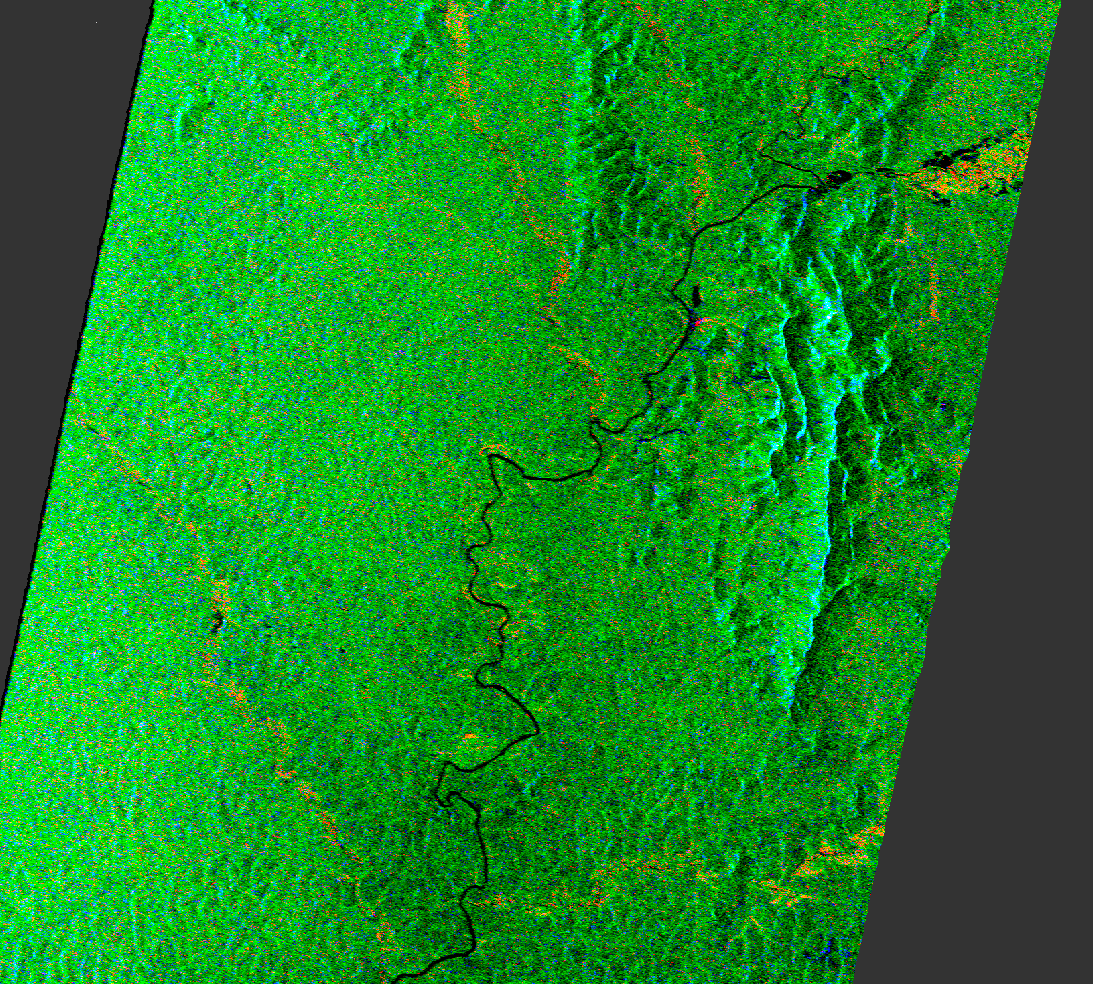
ESA SNAP 13 now includes the first generation of BIOMASS product support for ESA’s BIOMASS mission through the Microwave Toolbox. This is a useful step for researchers and SAR users who want to start testing workflows for the first spaceborne P-band SAR mission dedicated to measuring global forest biomass.
About ESA BIOMASS mission
ESA’s BIOMASS mission is introducing P-band SAR data into operational Earth observation workflows, with a strong focus on global forest biomass and forest height mapping. The long P-band wavelength can penetrate deep into forest canopies, which helps when analyzing forest structure and estimating above-ground biomass in dense vegetation regions.
Some of the main applications include:
· Above-ground biomass estimation
· Forest degradation and deforestation monitoring
· Forest structure analysis
· Carbon cycle and climate research
· Ecosystem modeling
P-band data may also be useful outside forestry applications. Potential applications also include wetland monitoring, geological mapping, and subsurface studies in dry regions.
Standard processing workflow for ESA BIOMASS data
The BIOMASS processing workflow in SNAP is similar to the one already used for Sentinel-1 products:
- Open and inspect the Level-1 product (Read operator) Load the BIOMASS product in SNAP Desktop, review the metadata, and examine the available polarization channels and image bands.
- Apply radiometric calibration (Calibration operator) Convert the SAR measurements into calibrated backscatter values such as Sigma0, Beta0, or Gamma0, depending on the analysis requirements.
- Terrain flattening (Terrain-Flattening operator, optional) In areas with strong topography, terrain flattening can help reduce radiometric effects caused by slope and viewing geometry.
- Terrain correction and geocoding (Terrain-Correction operator) Use a DEM to geocode the data and generate map-projected products suitable for further analysis or integration with GIS datasets.
- Export the results (Write operator) Processed outputs can be exported to formats such as GeoTIFF or NetCDF.
SNAP’s Graph Builder and GPF framework also make it possible to automate these workflows for batch processing or larger operational pipelines, including integrations with Python or HPC systems.
Polarimetric (PolSAR) workflow
Because BIOMASS is fully polarimetric, SNAP’s Radar → Polarimetric tools are central to most applications:
- Create/verify the polarimetric matrix. Use Polarimetric Matrix Generation to build the coherency (T3) or covariance (C3) matrix from the quad-pol channels.
- Polarimetric speckle filtering. Apply a matrix-preserving filter such as Refined Lee, IDAN or Lee Sigma to reduce speckle while keeping the polarimetric information intact.
- Polarimetric decomposition. Run the Polarimetric Decomposition operator to separate scattering mechanisms. Available methods include Pauli, Sinclair, Freeman-Durden, Yamaguchi, van Zyl, H/A/Alpha (Cloude-Pottier), Touzi, Krogager, Cameron and model-free 3-/4-component decompositions. For forests, Freeman-Durden/Yamaguchi (surface vs. double-bounce vs. volume) and H/A/Alpha (entropy/anisotropy/alpha) are the most informative.
- Classification (optional). Supervised or unsupervised polarimetric classification (e.g., Wishart H/A/Alpha) can segment forest, cleared land, regrowth and bare soil.
- Terrain correction + export as above.
Practical application of ESA BIOMASS data
Deforestation and Forest Degradation Monitoring using polarimetric tools
P-band’s penetration through the canopy to woody structure makes BIOMASS especially well suited to detecting not just outright clearing but also degradation (selective logging, thinning, fire damage), which optical sensors and shorter-wavelength radar often miss. The following multitemporal, polarimetry-based workflow detects and characterizes change:
- Build a multitemporal quad-pol stack. Read two or more BIOMASS Level-1 acquisitions over the same area, calibrate (Beta0) and coregister them into a common geometry.
- Polarimetric speckle filtering (Refined Lee) on each date’s T3/C3 matrix to stabilize the polarimetric estimates.
- Per-date polarimetric decomposition. Run Freeman-Durden/Yamaguchi and H/A/Alpha on each acquisition. Intact forest shows a dominant volume-scattering component with high entropy; clearing shifts the response toward surface scattering (low entropy, low alpha), while degradation produces an intermediate, declining volume contribution and changing double-bounce.
- Change detection. Differences between dates pinpoint loss and degradation:
- Drops in the volume-scattering fraction and HV backscatter flag canopy/biomass loss.
- Increases in double-bounce can indicate exposed trunks/regrowth structure.
- Interferometric coherence between dates adds a second, independent change signal: stable forest stays relatively coherent, whereas clearing causes a sharp coherence change.
- Classification and thresholding. Apply a Wishart or rule-based classification to the stacked decomposition + coherence layers to produce stable-forest / degraded / deforested classes.
- Terrain-correct, geocode and export the change map (GeoTIFF) for GIS overlay, validation against reference data, and area statistics.
메타데이터
- post_id
- 70eccf5efa3e
- slug
- native-biomass-support-in-esa-snap-13-70eccf5efa3e
- url
- https://medium.com/@esa.snap/native-biomass-support-in-esa-snap-13-70eccf5efa3e
- canonical_url
- https://medium.com/@esa.snap/native-biomass-support-in-esa-snap-13-70eccf5efa3e
- author_url
- https://medium.com/@esa.snap
- status
- ok
- fetched_at
- 2026-07-13 08:05:13
