美股ETF — VOO 與 QQQ 的選擇(Nasdaq-100 versus S&P500)

source: upslash by Anton

為什麼會要比較 VOO 與 QQQ

在選擇美股 ETF 時，通常會想到 VOO，因為 VOO 追蹤較為耳熟能詳的 S&P 500 指數，有些傾向更為分散的投資人，會選擇 VTI ，甚至是VT，畢竟 VTI 的公司分散程度更高，VT 還有跨國家。

如果希望追蹤大盤指數的話，其實 QQQ 所追蹤的 Nasdaq-100，也有其代表性，因此來比較與了解一下這兩支 ETF，做個紀錄。

要討論這兩檔 ETF，我想用他們追蹤的指數來分析

• S&P500
• Nasdaq-100

關於 S&P 500 指數

• 市值加權（float-adjusted market capitalization, FMC)(以在外流通股數為準）
• 最低市值要求為 $ 20.5B(2025/1/2)，這項要求是隨時間推進在改變的

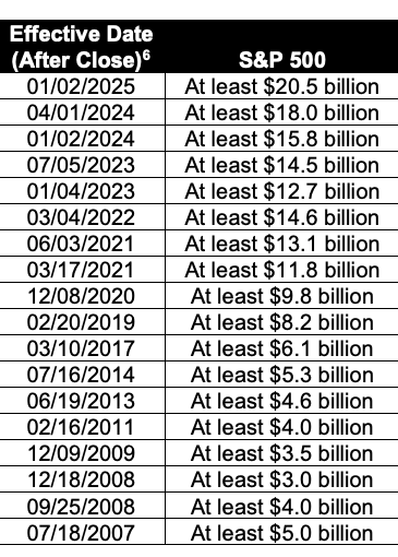
• 選擇市值前 500 大公司，可以跨交易所(NYSE, Nasdaq, Cboe)

關於 Nasdaq-100 指數

• 市值加權。
• Nasdaq Exchange 上市的股票挑前 100 大 ，而且必須非金融相關。
• 限制個股權重不能超過 24%，佔 4.5 %以上個股權重相加不能超過 48%。

兩檔指數都用市值做加權，而 Nasdaq 還增加了個股權重上限與避免過度集中的限制。

衡量報酬與風險

從下面的表格看到，報酬表現 Nasdaq-100 的累積報酬率完勝了 S&P 500，可以確定是來自於資金對於科技類股的追求，關於科技會不會一直是投資的主軸，以有限的未來來說，我認為仍然科技仍然會是引領市場的題材。

至於 Drawdown 在後面有比較多的討論。

Performance Comparison: NASDAQ-100 vs S&P 500
--------------------------------------------------------------------------------
Metric                                   NASDAQ-100              S&P 500
--------------------------------------------------------------------------------
Total Return (%)                            5299.83              1212.54
CAGR (%)                                      14.19                 8.94
Annualized Volatility (%)                     27.54                18.84
Maximum Drawdown (%)                          -82.9               -56.78
Sharpe Ratio                                   0.55                 0.44
Sortino Ratio                                  0.74                 0.57
Win Rate (%)                                  54.77                53.95

從圖來看就可以知道 2000 年當時的網路泡沫有多慘烈， Nasdaq-100 的 MDD 到 82.9%。

兩檔指數用 rolling 的情況來看兩者的 Volatility 和 Correlation，看到 Volatility 幾乎都是同向的變動，而兩者在報酬率的相關係數，則是在 Volatility 升高時會降低，Volatility 降低時會回升。

也就是說市場波動放大時，兩者表現相關性會降低，但綜觀來看，長期還是會維持 0.8 以上的水準。

關於風險 — 市場是否變得越來越健壯?

投資到現在，慢慢會開始在意可能的潛在風險，下面用三個時間點作為資料起始，分別為 1995 年, 2005 年與 2015 年，計算 Max Drawdown 在各個期間的變化，以及修復的時間。

計算的方法是，從資料起始點出現的第一個 Drawdown 為 Current Max Drawdown，紀錄發生日期與恢復時間(Recovery Time)，直到出現了大於 Current Max Drawdown 的 Drawdown 出現，就新增紀錄。

簡單說，新的 Drawdown 紀錄的幅度一定是比前一筆還要大。

先看到 1995 年，Nasdaq-100 指數在 2000 年的網路泡沫(dot-com bubble)出現了巨幅回檔，高達 82.9%，沒有實際經歷過當時的市場，很難想出現這種程度的跌幅，而這個 Drawdown 花了 4,775 天才在 2015–11–03 回到當時的水準，花了 13 年，是一個很震撼的數字。

S&P 500指數看起來在 2001 年也出現回檔，MDD 幅度僅管在金融海嘯時被刷新了，但恢復時間仍然是 2001 年花了比較久，用了 1,694 天，而金融海嘯的回撤則用了 1,480 天。

[Start Date 1995-01-01]

NASDAQ-100 Historical Maximum Drawdown Records:
----------------------------------------------------------------------------------------------------
Peak Date    Bottom Date    Peak Price    Low Price      MDD  Recovery Date  Recovery Days
----------------------------------------------------------------------------------------------------
1995-01-04   1995-01-05         399.65       398.02    0.41%     1995-01-06              1
1995-01-18   1995-01-30         419.26       401.71    4.19%     1995-02-06              7
1995-03-28   1995-04-06         460.54       439.92    4.48%     1995-04-26             20
1995-07-17   1995-07-19         596.91       547.12    8.34%     1995-09-07             50
1995-09-11   1995-10-09         609.75       546.93   10.30%     1995-11-02             24
1995-11-03   1996-01-09         621.71       534.42   14.04%     1996-02-08             30
1996-06-05   1996-07-23         699.35       598.34   14.44%     1996-09-13             52
1997-01-22   1997-04-02         925.52       783.92   15.30%     1997-05-05             32
1997-10-09   1997-12-24        1148.21       938.99   18.22%     1998-02-19             57
1998-07-20   1998-10-08        1465.89      1128.88   22.99%     1998-11-09             32
2000-03-27   2002-10-07        4704.73       804.64   82.90%     2015-11-03           4775

S&P 500 Historical Maximum Drawdown Records:
----------------------------------------------------------------------------------------------------
Peak Date    Bottom Date    Peak Price    Low Price      MDD  Recovery Date  Recovery Days
----------------------------------------------------------------------------------------------------
1995-01-04   1995-01-05         460.71       460.34    0.08%     1995-01-09              4
1995-01-17   1995-01-20         470.05       464.78    1.12%     1995-01-27              7
1995-02-24   1995-03-07         488.11       482.12    1.23%     1995-03-10              3
1995-05-16   1995-05-19         528.19       519.19    1.70%     1995-05-23              4
1995-07-17   1995-07-19         562.72       550.98    2.09%     1995-07-27              8
1995-10-19   1995-10-26         590.65       576.72    2.36%     1995-11-08             13
1995-12-13   1996-01-10         621.69       598.48    3.73%     1996-01-29             19
1996-02-12   1996-04-11         661.45       631.18    4.58%     1996-05-13             32
1996-05-24   1996-07-24         678.51       626.65    7.64%     1996-09-13             51
1997-02-18   1997-04-11         816.29       737.65    9.63%     1997-05-05             24
1997-10-07   1997-10-27         983.12       876.99   10.80%     1997-12-05             39
1998-07-17   1998-08-31        1186.75       957.28   19.34%     1998-11-23             84
2000-03-24   2002-10-09        1527.46       776.76   49.15%     2007-05-30           1694
2007-10-09   2009-03-09        1565.15       676.53   56.78%     2013-03-28           1480

接著把時間往後從 2005 年開始記錄，Nasdaq-100 與 S&P500 的 MDD 則都是受到金融海嘯影響，分別為 53.71% 與 56.78 ％，恢復時間分別花了 774 天與 1,480 天，大約是 2 年多和 4 年多。

[Start Date 2005-01-01]

NASDAQ-100 Historical Maximum Drawdown Records:
----------------------------------------------------------------------------------------------------
Peak Date    Bottom Date    Peak Price    Low Price      MDD  Recovery Date  Recovery Days
----------------------------------------------------------------------------------------------------
2005-01-03   2005-04-20        1603.51      1406.85   12.26%     2005-07-27             98
2006-01-11   2006-07-21        1758.24      1451.88   17.42%     2006-11-13            115
2007-10-31   2008-11-20        2238.98      1036.51   53.71%     2011-01-03            774

S&P 500 Historical Maximum Drawdown Records:
----------------------------------------------------------------------------------------------------
Peak Date    Bottom Date    Peak Price    Low Price      MDD  Recovery Date  Recovery Days
----------------------------------------------------------------------------------------------------
2005-01-03   2005-01-24        1202.08      1163.75    3.19%     2005-02-04             11
2005-03-07   2005-04-20        1225.31      1137.50    7.17%     2005-07-14             85
2006-05-05   2006-06-13        1325.76      1223.69    7.70%     2006-09-25            104
2007-07-19   2007-08-15        1553.08      1406.70    9.43%     2007-10-05             51
2007-10-09   2009-03-09        1565.15       676.53   56.78%     2013-03-28           1480

再往後 10 年到 2015 年， Nasdaq-100 的最大回撤為 35.56%，恢復時間僅花了 352 天，不到一年。S&P 500 則僅花不到半年就從疫情中的跌幅中爬回。

[Start Date 2015-01-01]

NASDAQ-100 Historical Maximum Drawdown Records:
----------------------------------------------------------------------------------------------------
Peak Date    Bottom Date    Peak Price    Low Price      MDD  Recovery Date  Recovery Days
----------------------------------------------------------------------------------------------------
2015-01-02   2015-01-06        4230.24      4110.83    2.82%     2015-01-08              2
2015-01-08   2015-01-15        4240.55      4089.65    3.56%     2015-01-22              7
2015-03-02   2015-03-11        4483.05      4305.38    3.96%     2015-04-24             44
2015-06-23   2015-07-08        4548.74      4351.58    4.33%     2015-07-16              8
2015-07-20   2015-08-25        4679.68      4016.32   14.18%     2015-11-02             69
2015-11-03   2016-02-09        4719.05      3947.80   16.34%     2016-07-28            169
2018-08-29   2018-12-24        7660.18      5899.35   22.99%     2019-04-17            113
2020-02-19   2020-03-20        9718.73      6994.29   28.03%     2020-06-05             77
2021-11-19   2022-12-28       16573.34     10679.34   35.56%     2023-12-15            352

S&P 500 Historical Maximum Drawdown Records:
----------------------------------------------------------------------------------------------------
Peak Date    Bottom Date    Peak Price    Low Price      MDD  Recovery Date  Recovery Days
----------------------------------------------------------------------------------------------------
2015-01-02   2015-01-06        2058.20      2002.61    2.70%     2015-01-08              2
2015-01-08   2015-01-15        2062.14      1992.67    3.37%     2015-01-22              7
2015-03-02   2015-03-11        2117.39      2040.24    3.64%     2015-04-24             44
2015-05-21   2016-02-11        2130.82      1829.08   14.16%     2016-07-11            150
2018-09-20   2018-12-24        2930.75      2351.10   19.78%     2019-04-23            119
2020-02-19   2020-03-23        3386.15      2237.40   33.92%     2020-08-18            148

從上面的數據觀察到，不論是 Nasdaq-100 還是 S&P 500，如果是越晚加入市場的投資人，可以享受到更強的市場修復能力，白話的說，以往害怕的黑天鵝事件，隨著時代演進、機制的完善與迅速的市場反應能力，導致投資人套牢的時間會逐漸減少。

結論

• 兩個指數高度相關的情況下，以追蹤指數為目標的 ETF，目前看來，其實擇一即可。
• 在市場修復能力變強的跡象看來，可以選擇 QQQ 作為美股的指數型 ETF 選擇。
• 後續還是要密切觀察科技主題是否維持在投資領域的熱度，現在看來沒有要退潮的跡象，也許是因為科技已經大面積的覆蓋人們的生活，而在技術上追求突破是沒有盡頭的一條路。

參考資料

[embed]S&P U.S. Indices Methodology | S&P Dow Jones Indices The S&P U.S. Indices are a family of equity indices designed to measure the market performance of U.S. domiciled stocks…www.spglobal.com

[embed]Nasdaq-100® | The Innovation Index for High-Growth Investments Invest in the Nasdaq-100®, the Innovation Index featuring top non-financial companies. Ideal for asset managers…www.nasdaq.com

程式碼

import yfinance as yf
import pandas as pd
import numpy as np
from datetime import datetime, timedelta
import matplotlib.pyplot as plt
import seaborn as sns

def get_index_data(ticker, start_date):
    """
    Fetch historical data for given index
    """
    index = yf.Ticker(ticker)
    df = index.history(start=start_date)
    return df['Close']

def calculate_historical_mdd_records(prices):
    """
    Calculate historical maximum drawdown records where:
    1. Each record represents a new deepest drawdown in history
    2. For each peak, only the maximum drawdown from that peak is considered
    """
    records = []
    historical_max_dd = 0
    running_peak = prices.iloc[0]
    running_peak_date = prices.index[0]
    current_peak_max_dd = 0
    current_peak_bottom_date = None
    current_peak_bottom_price = None

    def add_record(peak_date, bottom_date, peak_price, bottom_price, drawdown):
        future_prices = prices.loc[bottom_date:]
        recovery_dates = future_prices[future_prices >= peak_price].index
        recovery_date = recovery_dates[0] if len(recovery_dates) > 0 else None
        recovery_days = (recovery_date - bottom_date).days if recovery_date else None

        records.append({
            'Peak Date': peak_date.strftime('%Y-%m-%d'),
            'Bottom Date': bottom_date.strftime('%Y-%m-%d'),
            'Peak Price': round(peak_price, 2),
            'Low Price': round(bottom_price, 2),
            'MDD': round(drawdown, 2),
            'Recovery Date': recovery_date.strftime('%Y-%m-%d') if recovery_date else 'Not Yet',
            'Recovery Days': recovery_days if recovery_date else 'Ongoing'
        })

    for i in range(len(prices)):
        price = prices.iloc[i]
        date = prices.index[i]

        if price > running_peak:
            if current_peak_max_dd > historical_max_dd:
                historical_max_dd = current_peak_max_dd
                add_record(running_peak_date, current_peak_bottom_date, 
                          running_peak, current_peak_bottom_price, current_peak_max_dd)

            running_peak = price
            running_peak_date = date
            current_peak_max_dd = 0
            current_peak_bottom_date = None
            current_peak_bottom_price = None

        else:
            drawdown = (running_peak - price) / running_peak * 100
            if drawdown > current_peak_max_dd:
                current_peak_max_dd = drawdown
                current_peak_bottom_date = date
                current_peak_bottom_price = price

    if current_peak_max_dd > historical_max_dd:
        add_record(running_peak_date, current_peak_bottom_date,
                  running_peak, current_peak_bottom_price, current_peak_max_dd)

    return pd.DataFrame(records)

def calculate_performance_metrics(prices, risk_free_rate=0.02):
    """
    Calculate various performance metrics for a price series
    """
    # Calculate returns
    returns = prices.pct_change().dropna()

    # Basic metrics
    total_return = (prices.iloc[-1] / prices.iloc[0] - 1) * 100
    cagr = (prices.iloc[-1] / prices.iloc[0]) ** (252/len(returns)) - 1
    volatility = returns.std() * np.sqrt(252)

    # Maximum drawdown
    rolling_max = prices.expanding().max()
    drawdowns = (prices - rolling_max) / rolling_max
    max_drawdown = drawdowns.min() * 100

    # Risk-adjusted metrics
    excess_returns = returns - risk_free_rate/252
    sharpe_ratio = np.sqrt(252) * excess_returns.mean() / returns.std()
    sortino_ratio = np.sqrt(252) * excess_returns.mean() / returns[returns < 0].std()

    # Win rate
    win_rate = (returns > 0).mean() * 100

    return {
        'Total Return (%)': round(total_return, 2),
        'CAGR (%)': round(cagr * 100, 2),
        'Annualized Volatility (%)': round(volatility * 100, 2),
        'Maximum Drawdown (%)': round(max_drawdown, 2),
        'Sharpe Ratio': round(sharpe_ratio, 2),
        'Sortino Ratio': round(sortino_ratio, 2),
        'Win Rate (%)': round(win_rate, 2)
    }

def plot_index_comparison(nasdaq_prices, sp500_prices):
    """
    Create comparison plots for the indices using cumulative returns
    """
    # Calculate cumulative returns
    nasdaq_returns = nasdaq_prices.pct_change()
    sp500_returns = sp500_prices.pct_change()

    nasdaq_cum_returns = (1 + nasdaq_returns).cumprod() - 1
    sp500_cum_returns = (1 + sp500_returns).cumprod() - 1

    # Create figure with subplots
    fig = plt.figure(figsize=(15, 10))

    # Cumulative Returns Plot
    ax1 = plt.subplot(2, 1, 1)
    ax1.plot(nasdaq_cum_returns.index, nasdaq_cum_returns * 100, label='NASDAQ-100', color='blue')
    ax1.plot(sp500_cum_returns.index, sp500_cum_returns * 100, label='S&P 500', color='red')
    ax1.set_title('Cumulative Returns')
    ax1.set_ylabel('Cumulative Return (%)')
    ax1.legend()

    # Drawdown Plot
    ax2 = plt.subplot(2, 1, 2)
    nasdaq_dd = (nasdaq_prices - nasdaq_prices.expanding().max()) / nasdaq_prices.expanding().max() * 100
    sp500_dd = (sp500_prices - sp500_prices.expanding().max()) / sp500_prices.expanding().max() * 100

    ax2.fill_between(nasdaq_dd.index, nasdaq_dd, 0, alpha=0.3, color='blue', label='NASDAQ-100')
    ax2.fill_between(sp500_dd.index, sp500_dd, 0, alpha=0.3, color='red', label='S&P 500')
    ax2.set_title('Drawdown Comparison')
    ax2.set_ylabel('Drawdown (%)')
    ax2.legend()
    ax1.spines['top'].set_visible(False)
    ax1.spines['right'].set_visible(False)
    ax2.spines['top'].set_visible(False)
    ax2.spines['right'].set_visible(False)
    ax1.grid(axis='y', linestyle='--', alpha=0.7)
    ax2.grid(axis='y', linestyle='--', alpha=0.7)
    plt.tight_layout()
    fig.savefig('index_comparison.png', dpi=300)
    plt.show()

def plot_rolling_metrics(nasdaq_prices, sp500_prices, window=252):
    """
    Plot rolling volatility and correlation
    """
    # Calculate daily returns
    nasdaq_returns = nasdaq_prices.pct_change().dropna()
    sp500_returns = sp500_prices.pct_change().dropna()

    # Calculate rolling metrics
    rolling_vol_nasdaq = nasdaq_returns.rolling(window).std() * np.sqrt(252) * 100
    rolling_vol_sp500 = sp500_returns.rolling(window).std() * np.sqrt(252) * 100
    rolling_corr = nasdaq_returns.rolling(window).corr(sp500_returns)

    # Create figure with subplots
    fig = plt.figure(figsize=(15, 10))

    # Rolling Volatility
    ax1 = plt.subplot(2, 1, 1)
    ax1.plot(rolling_vol_nasdaq.index, rolling_vol_nasdaq, label='NASDAQ-100', color='blue')
    ax1.plot(rolling_vol_sp500.index, rolling_vol_sp500, label='S&P 500', color='red')
    ax1.set_title(f'Rolling {window//252}-Year Annualized Volatility')
    ax1.set_ylabel('Volatility (%)')
    ax1.legend()

    # Rolling Correlation
    ax2 = plt.subplot(2, 1, 2)
    ax2.plot(rolling_corr.index, rolling_corr, color='purple')
    ax2.set_title(f'Rolling {window//252}-Year Correlation')
    ax2.set_ylabel('Correlation')

    ax1.spines['top'].set_visible(False)
    ax1.spines['right'].set_visible(False)
    ax2.spines['top'].set_visible(False)
    ax2.spines['right'].set_visible(False)
    ax1.grid(axis='y', linestyle='--', alpha=0.7)
    ax2.grid(axis='y', linestyle='--', alpha=0.7)
    plt.tight_layout()
    fig.savefig('rolling_metrics.png', dpi=300)
    plt.show()

def format_drawdown_table(df, index_name):
    """
    Format drawdown records into a pretty table
    """
    print(f"\n{index_name} Historical Maximum Drawdown Records:")
    print("-" * 100)
    print(f"{'Peak Date':<12} {'Bottom Date':<12} {'Peak Price':>12} {'Low Price':>12} "
          f"{'MDD':>8} {'Recovery Date':>14} {'Recovery Days':>14}")
    print("-" * 100)

    for _, row in df.iterrows():
        print(f"{row['Peak Date']:<12} {row['Bottom Date']:<12} {row['Peak Price']:>12.2f} "
              f"{row['Low Price']:>12.2f} {row['MDD']:>7.2f}% {str(row['Recovery Date']):>14} "
              f"{str(row['Recovery Days']):>14}")

def format_performance_comparison(metrics1, metrics2, name1, name2):
    """
    Format performance comparison table
    """
    print(f"\nPerformance Comparison: {name1} vs {name2}")
    print("-" * 80)
    print(f"{'Metric':<30} {name1:>20} {name2:>20}")
    print("-" * 80)

    for metric in metrics1.keys():
        print(f"{metric:<30} {metrics1[metric]:>20} {metrics2[metric]:>20}")

def main():
    # Set style for plots

    # Define parameters
    start_date = "1995-01-01"
    nasdaq_ticker = "^NDX"  # NASDAQ-100 ticker
    sp500_ticker = "^GSPC"  # S&P 500 ticker

    # Fetch data
    nasdaq_prices = get_index_data(nasdaq_ticker, start_date)
    sp500_prices = get_index_data(sp500_ticker, start_date)

    # Calculate drawdowns
    nasdaq_drawdowns = calculate_historical_mdd_records(nasdaq_prices)
    sp500_drawdowns = calculate_historical_mdd_records(sp500_prices)

    # Calculate performance metrics
    nasdaq_metrics = calculate_performance_metrics(nasdaq_prices)
    sp500_metrics = calculate_performance_metrics(sp500_prices)

    # Display results
    format_drawdown_table(nasdaq_drawdowns, "NASDAQ-100")
    format_drawdown_table(sp500_drawdowns, "S&P 500")
    format_performance_comparison(nasdaq_metrics, sp500_metrics, "NASDAQ-100", "S&P 500")

    # Create visualizations
    plot_index_comparison(nasdaq_prices, sp500_prices)
    plot_rolling_metrics(nasdaq_prices, sp500_prices)

if __name__ == "__main__":
    main()