Everything Is Radio: Mapping the Invisible Airwaves with a Borrowed Dongle and an AI Partner
What a borrowed $25 radio receiver, a random antenna, and an AI partner can teach you about the electromagnetic world hiding in your walls.
Everything Is Radio: Mapping the Invisible Airwaves with a Borrowed Dongle and an AI Partner
What a borrowed $25 radio receiver, a random antenna, and an AI partner can teach you about the electromagnetic world hiding in your walls.
by yoyoerx, with Claude Code (Anthropic) as shadow author
There is a moment, early in any radio experiment, that is genuinely disorienting. You plug in a small USB device, point an antenna at the ceiling, and suddenly you are looking at a waterfall display lit up like a city from 30,000 feet. Streaks of color scroll past — some constant and bright, some flickering, some appearing for a fraction of a second and gone. The air around you, the same air you just breathed, is full of signals. They were always there. You just couldn’t see them.
I borrowed an RTL-SDR dongle from work for a weekend project. One of those situations where you say “I’ll have it back Monday” and then Monday becomes a month because you can’t put it down. What I didn’t expect was what would happen when I paired it with Claude Code and started asking questions.
The Hardware
The RTL-SDR is not impressive hardware. It is a repurposed digital television chip — the Realtek RTL2832U, designed to decode DVB-T broadcasts — that some clever engineers noticed could be put into a raw I/Q sample mode. In that mode it becomes a general-purpose software-defined radio receiver covering roughly 24 MHz to 1766 MHz. No specialized antenna. No filtering. No front-end protection. Just raw samples, streaming off the USB bus at up to 2.4 million samples per second, waiting for software to make sense of them.
The antenna I had on hand was a random rubber duck pulled from a drawer — probably tuned somewhere around 900 MHz, though with rubber ducks you can never really be sure. It picks up everything badly and unevenly. Which, for exploration, turns out to be fine. You are not trying to receive cleanly. You are trying to see what is there.

The waterfall display — each horizontal line is one FFT snapshot; time scrolls downward. The bright vertical streaks are signals
Building Instead of Borrowing
The obvious move would be to install SDR#, fire it up, and call it a day. I did not do the obvious thing. I wanted to understand what was actually happening — not just look at it — and that meant building the tools with Claude Code as my co-pilot.
What started as a Python script to stream IQ samples and compute an FFT became something else entirely over a few sessions. A scrolling waterfall display. A headless scanner that could sweep the whole spectrum while I slept. A review application for browsing and labelling what it found. A signal family analyzer that could detect the stereo pilot tone, RDS data subcarrier, and HD Radio sidebands on an FM broadcast signal and label them correctly as a family. A SQLite database to hold everything.
This is the part that is hard to convey unless you have used Claude Code this way: the conversation moves fast. Not “fast” like autocomplete. Fast like having a domain expert in the room who has read every RF textbook, can hold the full context of what you have built so far, and asks the right clarifying questions before writing a line of code. You describe what you want to understand, it helps you figure out how to see it, and the tools that emerge from that process are shaped by curiosity rather than by copying an existing workflow.
What the Spectrum Actually Looks Like
Once you can see it, the first thing you notice is how much is happening in the FM broadcast band. The stretch from 88 to 108 MHz, over any major metropolitan area, is a wall of signals. Thirty or more stations, most of them stronger than anything else in the entire spectrum. But look more closely — zoom in on a single strong station — and you start to see structure. Symmetrical lobes 38 kHz out from the carrier. Narrower spikes 57 kHz out. Faint OFDM sidebands 100 to 200 kHz away on the strongest stations. The stereo subcarrier, the RDS data channel, the HD Radio digital layer. A single FM broadcast transmission is not one signal. It is five.

One FM broadcast station, zoomed in. The main carrier is in the center; the lobes and spikes around it are the stereo subcarrier, RDS data channel, and HD Radio digital layer
Above 108 MHz, the aviation band begins. This is where the air gets interesting in a different way. Between 118 and 136 MHz, every frequency that carries a signal is a voice channel for an aircraft or a controller. Most of them are quiet most of the time — you are hearing empty carrier, the radio left keyed — but occasionally a burst of audio-modulated signal appears, peaks, and is gone. At 129 MHz you can see the ACARS digital datalink: narrow chirps, faster than voice, carrying aircraft position and maintenance data. At 136.65 and 136.9 MHz, VDL Mode 2 digital packets.
At 144.390 MHz there is almost always something. APRS — the Automatic Packet Reporting System — is a network of amateur radio operators transmitting position reports, weather observations, and messages using 1200-baud Bell 202 audio-frequency shift keying on a standard NFM voice channel. The bursts are short and loud and unmistakable once you have seen a few.
At 433 MHz, the ISM band smells like a neighbourhood. Short bursts from tire pressure monitors. Longer FSK chirps from wireless weather stations. OOK blinks from key fobs and doorbell buttons. These are not signals from infrastructure. They are signals from people’s driveways and garages and front porches.
At 902 MHz, something unexpected: dense IoT traffic. LoRa uplink packets, spaced 200 kHz apart across the whole US sub-band, arriving continuously. Smart meters, soil sensors, asset trackers, Helium network nodes. The Internet of Things is not a metaphor. It is a literal electromagnetic fog covering every neighborhood, and most people standing in it have no idea it exists.
At 1090 MHz, ADS-B. Every commercial aircraft transponder broadcasting its position, altitude, velocity, and identity at roughly once per second. The signal is short — 120 microseconds — and arrives as a persistent elevated carrier in the averaged spectrum because dozens of aircraft are transmitting simultaneously. You cannot decode individual messages from a bulk capture at this resolution, but you can watch the band light up and dim as traffic patterns shift through the day.
The Classifier That Lied
This is where I have to be honest about a failure, because it is instructive.
The goal from the beginning was to build a machine learning classifier — train a RandomForest model on labeled captures, run it in the scanner, and have every detected signal automatically identified. It seemed like the natural next step after building a signal library.
It worked, in the narrow sense. The model trained cleanly. Five-fold cross-validation showed 92.1% accuracy. Out-of-bag score 92.4%. I integrated it into the scanner, ran a full 24–1766 MHz sweep, and went to bed.
The next morning the database had over a thousand new ML-labeled captures. And they were wrong. Not subtly wrong — confidently, absurdly wrong. Aviation voice at 512 MHz. FM broadcast at 548 MHz. ISM 900 LoRa at 51 MHz. ADS-B at 51.5 MHz. The average confidence on these labels was 58 to 66 percent — just high enough to look like the model knew what it was doing.

The seven signal classes the RandomForest was trained on, shown against the full tunable range of the RTL-SDR. Everything outside those bands was unknown territory to the model — but the model had no way to say so.
The problem was not the model. The model was doing exactly what it was trained to do: given a signal with certain spectral features, return the closest label from among the seven classes it had seen. The problem was that the training set covered seven bands out of a spectrum that spans 1700 MHz. Every signal the model had never seen — unknown pagers, unlicensed devices, harmonics, intermodulation products — got classified as the closest thing in its vocabulary. The model had no “I don’t know.” It had no concept of out-of-distribution input. It had learned to categorize the familiar and was silently, confidently hallucinating labels for everything else.
The fix was surgical. Every label assigned by the ML scanner — 1,088 of them — was cleared from the database. The confidence column in the captures table is the provenance marker: non-null means the scanner ML assigned it, null means a human or the frequency-heuristic autolabeler assigned it. Removing the bad labels left 715 correctly labeled captures and 919 honestly unlabeled ones.
The scanner’s default was changed: it no longer loads or uses the classifier by default. Labels are now assigned after scanning by a frequency-heuristic tool, which uses band allocation rules — rules that are always right about which frequency a signal is in, because that is a physical fact, not a prediction.
The ML approach itself is being rethought from the ground up. The RandomForest was a reasonable first pass, but the failure revealed a deeper architectural problem: a classifier that cannot express uncertainty is not a classifier, it is a label dispenser. Whatever comes next — and Claude and I haven’t settled on an approach yet — it needs to know what it doesn’t know. That is the design constraint the failure gave us, and it is a better starting point than any amount of cross-validation accuracy would have been.
What Human-Machine Teaming Actually Means Here
The standard framing for AI-assisted development is productivity: you write faster, you ship sooner, you handle more tickets. That framing misses what was actually happening in these sessions.
Claude Code was not just generating code. It was helping me develop a mental model of a domain I did not know. When I described a signal I was seeing — narrow, 4 kHz wide, near 144 MHz, appearing in brief bursts — and asked what it might be, the answer was not just “APRS.” It was an explanation of Bell 202 AFSK, why the frequency offset produces the characteristic double-hump PSD shape, what the ±1 kHz subcarriers represent, and why the apparent center frequency drifts around 144.390 MHz instead of sitting still (RTL-SDR LO offset, not a correctable PPM error — there are two distinct offset clusters in the data, which rules out a single-value correction). That is not productivity. That is learning.
The tools we built together were shaped by the questions I was asking. The signal family analyzer exists because I wanted to understand why FM broadcast looked so wide. The per-peak classifier exists because I wanted to know which of the dozen signals visible in a 2.4 MHz window was which — not just “the loudest one.” The power history mode in the time domain panel exists because I wanted to watch a quiet aviation channel and see when it woke up, not just whether it was active in the current frame.
None of these features appear on a requirements list. They emerged from curiosity meeting capability.
And when the classifier failed, the diagnosis was a conversation too. Not “here is what went wrong” delivered as a report. More like two people looking at the same evidence and working out together why something that looked correct had gone badly wrong, and what the right constraints were for the next attempt. The failure became part of the shared context. The next architecture will be built with that failure explicitly in mind.
That is the part that is hard to replicate with any other tool. Not the code generation. The continuity of understanding.
What I Know Now That I Did Not Know Then
The air over any major metropolitan area is carrying, at any moment:
- Dozens of broadcast stations, each transmitting multiple parallel signals
- Hundreds of aviation voice channels, most of them silent
- Digital datalinks moving aircraft position and maintenance data
- Amateur radio operators sending position reports via a protocol designed in the 1990s
- Tens of thousands of IoT devices quietly reporting to servers they will never meet
- Pager networks, still operating, still carrying messages to people who rely on them
- Every aircraft overhead announcing its position to anyone listening
None of this requires special access. No license to receive. No expensive equipment. A borrowed dongle, a rubber duck antenna from a drawer, and software you can build in a weekend.
What it does require is a way to make sense of what you hear. That is the part that changed with this project. Not the hardware — the hardware has been available for over a decade. The AI companion that can hold the full context of what you are building, explain the physics when you need it, catch the bugs before they corrupt a thousand database records, and sit with you through a failure until you understand it well enough to do better next time.
The electromagnetic world was always there. It just needed the right partner to help see it.
yoyoerx writes about hardware exploration, signal intelligence, and human-AI collaboration. Follow on Medium at @yoyoerx.
This article was co-written with Claude Code (Anthropic), which served as co-architect of every tool described here, domain expert across RF, DSP, and software design, and shadow author of this piece. The project was built entirely through conversation — no formal specification, no design doc, just questions meeting capability across many sessions.
Tags: Artificial Intelligence · Machine Learning · Programming · Internet Of Things · Signal Processing
메타데이터
- post_id
- 77b9e1bcf0ff
- slug
- everything-is-radio-mapping-the-invisible-airwaves-with-a-borrowed-dongle-and-an-ai-partner-77b9e1bcf0ff
- url
- https://radiohackers.com/everything-is-radio-mapping-the-invisible-airwaves-with-a-borrowed-dongle-and-an-ai-partner-77b9e1bcf0ff
- canonical_url
- https://radiohackers.com/everything-is-radio-mapping-the-invisible-airwaves-with-a-borrowed-dongle-and-an-ai-partner-77b9e1bcf0ff
- author_url
- https://medium.com/@yoyoerx
- status
- ok
- fetched_at
- 2026-06-16 19:09:56