Computer Vision: Key Point Detectors and Feature Descriptors — Part 2
In the last part, we talked about edges and corners. While these are useful as local features, blobs (small areas) are generally more…
Computer Vision: Key Point Detectors and Feature Descriptors — Part 2
In the last part, we talked about edges and corners. While these are useful as local features, blobs (small areas) are generally more helpful in computer vision tasks.

A blob has a fixed position and size in the image. For a blob to be useful, we need to locate the blob, determine its size, determine its orientation, and finally, formulate a description or signature for that blob that is independent of size or orientation.
Blob Detection
Blob detectors can be built by extending the basic edge detector idea that we discussed previously. Let’s first look at 1D blobs and see what happens when they pass through a LoG filter:

You can see that it generates different types of responses depending on how wide the input signal is. So what can we do? We apply what’s known as scale normalization — where we multiply the Gaussian kernel response by its variance σ².

This operator is called the Normalized Laplacian of Gaussian (NLoG). At some value of σ, the responses show a peak. Now, in order to find a blob, all we have to do is get the responses for multiple values of σ and find the local extrema.
We also define a term called the characteristic scale as the scale that produces maximum response at the location of the blob:

In this image, our original candidate blob signal is on the left. On the right, we have its Laplacian response after scale normalization for a series of different σ. We see that the maximum response comes at σ=8, so we say the characteristic scale is at σ=8.
Watch what happens to the Laplacian response as we vary σ without scale normalization:

As you can see, we don’t get the maximum response at σ=8
The above concept is very easy to extend to 2D, by taking the partial derivatives w.r.t. both x and y.

We previously mentioned taking the responses for multiple σ values. This set of values is called the Scale space.

It’s possible to prove that for a binary circle of radius r, the Laplacian achieves a maximum at σ = r/√2:

SIFT Detector
Let’s say you want to map the following object to the image on the right:

It’s rotated, has a different scale, and is even obstructed by other objects. So how can you do this? As we already discussed, we can match the important features (blobs) of the object to the image. That’s exactly what the SIFT detector does.
The Scale Invariant Feature Transform (SIFT) Detector is very widely used. What makes it so reliable is that it uses a few mathematical tricks. One such trick is NLoG approximation:

Previously we used the NLoG operator for blob detection. Turns out we can take the difference of 2 Gaussians of the image, and that gives a pretty good approximation to the NLoG operator.
This is very useful, because now rather than computing NLoG for the scale space (entire stack of scaled images), which is computationally expensive, we can just take any 2 consecutive images and find the Difference of Gaussian (DoG) between them.
Let’s see how SIFT is implemented end-to-end:

First step is to create the stack of images by applying different scale normalizations and obtaining the scale space.
Then, using the DoG, we approximate the NLoG filter. Next, we find the local extremas by using a 3x3 window and shifting it throughout the image.
After we do that, we get our interest points. These are the candidates for our SIFT features. Since we may have too many of them, we can use a thresholding to preserve only the strongest extremas, and now we have our result:

Each of these circles corresponds to an extracted SIFT feature. So now we have found the interest points, with their locations and scales. We can use this information to transform the features of the object to match the features in the image.
Let’s say that the following blob (denoted in blue) occupies a grid of pixels in the image:

For every pixel in the grid, you’re going to apply the gradient operator, which gives you the magnitude and the orientation of the pixel. We’re going to ignore the magnitude because the magnitude is affected by lighting, shadows, etc. So we only care about the orientations.
Using the orientation values, we can create a histogram where on the x-axis we can have the different directions of the gradient, and the y-axis corresponds to the number of pixels in that direction:

We can then take the most prominent direction (the principal orientation) and use this to transform the rotation based on our object:

So we have undone the effects of rotation, our filter is already insensitive to scale, and since we didn’t consider the magnitude, we are not affected by things like brightness. This makes the SIFT detector invariant to brightness, scale and rotation.
What actually happens in SIFT is that the pixel grid covered by a blob is divided to 4 quadrants, and their gradient orientation histograms are plotted separately:

This is called the SIFT descriptor — a 128-dimensional vector representing the gradient orientations around a blob. Once we obtain this vector for both our image and target object, we need to compare them to find the corresponding points between the image and object. For this we have a couple of options:
- L2 distance / Sum of squared differences (SSD)

- Normalized correlation — dot product between 𝒖 and v normalized to have zero mean and unit norm:

The normalized correlation is more preferred because it provides superior robustness to changes in image illumination, contrast, and gain.
References
https://courses.cs.washington.edu/courses/cse455/24sp/slides/08_detectors_and_descriptors.pdf
[embed]
메타데이터
- post_id
- 77f04eb8cfad
- slug
- computer-vision-key-point-detectors-and-feature-descriptors-part-2-77f04eb8cfad
- url
- https://medium.com/@ckekula/computer-vision-key-point-detectors-and-feature-descriptors-part-2-77f04eb8cfad
- canonical_url
- https://medium.com/@ckekula/computer-vision-key-point-detectors-and-feature-descriptors-part-2-77f04eb8cfad
- author_url
- https://medium.com/@ckekula
- status
- ok
- fetched_at
- 2026-06-21 15:33:18