QuickBooks: Top Sales by category prediction system for customer [training millions of model daily]

Part 2 of this doc will tackle the GTM strategy with a scalable and customisable subscription model.

1. Introduction

QuickBooks is a multi-tenant commerce platform designed to help small and medium-sized businesses manage their financial operations. It enables customers to create and manage product and service catalogs, organise them into categories, and track sales activity. The platform provides analytical reports such as Sales by Product/Service Summary, allowing users to identify top-performing offerings and gain insights into their overall business performance. These insights support data-driven decisions across inventory planning, pricing strategies, and marketing optimization.

2. Background / Context

QuickBooks Commerce users lack a scalable and accurate mechanism to forecast their future top-selling products and revenue across categories. Without reliable forecasts, users struggle to proactively plan inventory, optimise pricing, and align marketing efforts. There is a need for a robust forecasting and ranking system that provides actionable, forward-looking insights to support business planning and decision-making.

3. Goals

1. Design and implement a scalable, high-performance forecasting and ranking system that delivers “top sales by category” predictions across multiple time horizons (next week, next month, next year) for approximately 10 million tenants(a term used synonymously with customers).

2. The system should efficiently handle tenant-specific product catalogs, category structures and sales behaviours while ensuring high accuracy, low latency, and operational reliability at scale.

Out of scope:

• Building or maintaining a global product taxonomy system, including ML-based classification and human review workflows.
• Providing real-time streaming predictions. All forecasting and ranking will operate in batch mode with periodic refresh.
• Providing SKU-level forecasting. The system focuses on category-level ranking and forecasting, not individual product prediction.
• Developing customer-specific custom models or tuning workflows. Forecasting and ranking models will follow standardised training and deployment pipelines.

4. Assumptions

1. We assume the existence of a normalised category taxonomy (“Category_Group”) that maps tenant-specific category_id and product_id values to a consistent global category structure. A taxonomy mapping solution (e.g., SIC/NAICS alignment using ML classification and human review workflows) is feasible, it introduces significant complexity and operational overhead. To keep the system scope focused and tractable, we assume that a reliable Category_Group mapping is already available.

2. Daily aggregated sales data is reliable, complete and available as a fact table/data source.

• Existing capability in QB to generate daily sales reports.
• Alternatively, it will require us to set up CDC based event processing pipeline that executes complex accounting logic to reconstruct daily sales per tenant from raw transactional data including refunds, partials, currency normalisation and taxes. Implementing such a pipeline is out of scope of this doc.

3. Holiday calendars are available by region.

4. Scale: +10M Customers with average 500 SKUs spread across 30 categories

5. Requirements Summary

Functional Requirements:

1. Users will be able to enable “Top Selling by category” by revenue or units sold feature on their QB dashboard.
2. Users will be able to see the top 5 “Top selling category”.
3. Users will be able to toggle between Next Week, Next Month and Next Year forecast views.
4. UI will be able to select one of the top categories and it will render a graph with clear visual boundary between historical “Actuals” and “Forecasted” values.
5. UI shall display a probabilistic confidence band (shaded region) around the primary forecast line to represent prediction uncertainty.
6. UI shall display a high visibility badge indicating confidence_level for forecast of selected category.
7. As new daily sales data becomes available, the system shall convert the previous day’s forecasted values into historical “Actuals”, enabling users to visually compare predicted vs. actual performance.

Non-Functional Requirements:

1. Prefer availability over consistency for forecasts outputs and fallback to statistical calculations.
2. Latency: Graphs should render in < 200ms @P95 of initial page load time.
3. Scalability: system should scale horizontally to support >= 10MM customers, billions of records and millions of model training jobs without architectural changes.
4. The end-to-end model training pipeline should complete within Tk hours to support daily refresh cycles at full system scale.
5. Accuracy & Quality: Capture and monitor standard metrics like MAPE, MAE, RMSE, Bias and Top-K Revenue Capture etc.
6. Fault tolerance & Resilience: Training and data processing pipelines should be fault tolerant supporting automatic retries, partial job recovery and failure isolation at tenant and task granularity.
7. Monitoring: system should provide end to end observability on pipeline health, training progress, failure rates, data freshness indicators and forecast accuracy metrics.
8. Security & Privacy : comply with GDPR and internal security standards including data encryption at rest and in transit, access control and isolation by tenancy and anonymisation for aggregated analytics.
9. Auditability: system should retain historical forecasts and actuals for model evaluation, debugging and business audits.
10. Backward compatibility: changes to forecasting models should not break dashboards.
11. Deployments, Rollback: system should support model rollouts, with versioning, canary testing and fast rollbacks on degradation.
12. Experimentation and CI: system should support A/B testing, enable side by side evaluation of model versions, offline backtesting and online shadow testing without impacting production customers.

6. Proposal

QB serves ~10MM customers, each with distinct product catalogs, category structures and sales patterns. This creates a highly heterogeneous tenant behaviour which has to be addressed at scale. The diverse set of customers ranges from “New Tenants” that lack historical data to “Mature tenants” exhibiting strong seasonal patterns implying that a single modelling approach cannot work uniformly.

In order to predict the top Sales category for Cold start Tenants, we can leverage global priors driven by population like category trends, regional behaviour and cohort level statistics. While for mature tenants the system will use time series historical data to forecast with models like SARIMA and Prophet for the required time horizons.

We propose using a maturity-aware unified scoring system that addresses aforementioned challenges:

Score:= w1 short_term_velocity + w2 trend_strength + w3 forecasted_revenue + w4 category_prior

This blends in a weighted combination of a) recent momentum specific to the tenant, b) emerging demand patterns at cohort level, c) long term tenant specific demand with increasing reliability with time and d) global and regional market behaviour (critical for cold start tenants).

Forecasting models will be trained per tenant while for the weights instead of hand picked values we will set up a Gating Network using a Linear regression model that looks at the customer’s age to decide weights.

7. High level architecture

At high level, system functionality is broken into 4 managed layers each managing its own complexity:

1. Data Ingestion and Transformation layer

We will use spark job that runs once everyday and ingests daily revenue and unit sales data from upstream fact tables for all customers, categories and SKUs. Additionally it will normalise timestamps and currencies, validating data quality before writing to S3 folder paths.

2. Feature Engineering Layer

A park job will fetch normalised datasets from layer 1 to enrich dataset with the model ready features like a) rolling aggregates last_3d, last_7d, prev_7d , last_30d, prev_30d revenue, b) calendar features holidays, day_of_the_week, days_to_holiday, is_holiday. c) growth signals rev_growth_7d, rev_growth_30d d) velocity signals : velocity_3_14, velocity_7_30. e) Category Priors (global and regional aggregation). Details are provided in the next sections.

3. Model Training Layer

3.1. Forecast Models Pipeline:

Responsible for learning tenant-level demand patterns and producing future revenue predictions across time horizons. The system will adapt forecasting based on Customer-category temporal history. Seasonality aware models like SARIMA/Prophet will be used for mature time series while a cohort level LightGBM model will be used to generate forecasts for all three horizons. This ensures long range projections are stable while customer responsiveness is preserved without incurring the cost of retraining millions of full series models too quickly.

There will be a need to smoothen out this model transition so the Customer doesn’t see a totally different graph between day 180 and 181. We will use a smoothening factor w to define the forecast function as this: F_final​(t) = w⋅F_prophet​(t)+(1−w)⋅F_lgbm​(t). The value of w changes between 0 to 1 over time.

Following is a high level proposal on training cadence for the models involved in forecasting. This will be completely configuration based and downstream layers need not be aware of this. Furthermore, not all M million Prophet models have to be trained in a single batch on the same day. It will be a scheduled rolling batch based on the last training-date for a customer-category.

Given the scale of customers which is expected to increase at the rate 8–10% YOY, training these models requires massively parallel execution infrastructure that’s fault tolerant. We will set up a distributed batch pipeline orchestrated by Airflow and combination of Ray and Kubernetes as execution engine for horizontally scalable parallelism, dynamic resource scheduling, automatic retries of failed tasks and distributed task graph execution of python workloads for inference and ML training workloads.

Closest alternative is Sagemaker pipelines with warm pools but at scale of 10M small models, Ray’s actor model avoids container startup overhead and allows for a cost-effective use of spot instances.[refer section 12 for comparison]

As an industry standard will use MLflow as the model governance and experiment tracking layer integrated into Ray workers. From model metric logging and accuracy monitoring (MAPE, WAPE, Bias, RMSE, Top K revenue capture etc) to registry and version control, MLFlow will provide the audit trail for predictions served on QuickBooks UI.

3.2. Linear Regression (LR) Model pipeline:

To account for heterogeneous tenant maturity, the system trains three independent regression models, each optimised for a different data segment :

For training dataset construction, we will select datasets of tenants(and category) having more than 2 years of historical data

For each such tenant:

1. Select multiple historical cut-points T (referring to phase as defined above).
2. Generate feature vectors using the data up to T. (as defined in feature engineering layer)
3. Compute label using actual realised revenue from(T+1 -> T + horizon)

This would yield millions of supervised training samples for each of the segments defined above. Except the forecast models’ predictive signals, rest of all feature calculations are one time for one Golden dataset (e.g. velocity, trend, prior, actual_future_revenue etc). Hence for each regression retrain cycle, we will generate fresh forecast values and inject into the dataset before retraining the LR model.

We will use similar infrastructure as defined for Forecast model training with a retrain cycle as monthly or quarterly. Three segments capture the transition of a customer from cold -> growing or growing to mature, so weekly or monthly re-trainings will only add operational burden rather than improving performance/accuracy of model.

4. Serving and Visualisation layer

Primary (Durable) Storage:

Nightly scoring (i.e. Top Sales by Category pre-computation) jobs are triggered from a separate Airflow DAG, either immediately followed after an async training job or as a fixed nightly job.

The Ray cluster can remain warm to minimise startup latency and maximise cost efficiency. Scoring engine pulls the “Champion” models and writes the ranked category list (top 5) and forecast data points for UX to low latency and scalable data stores.

Outputs:

a). Ranked category list per customer

Schema: (customerId (primary key), ranking#{timeframe} (sort key) . e.g. week, month, year)

b). Forecast Data points

Schema: customerId#category_id (primary key), dateTime (Sort key)

8. Detailed Design

8.1 Airflow Orchestration layer

Central control plane for batch workflows, dependencies, retries and observability. We will use Airflow Scheduler, web UI and workers. Recommendation is to use a managed Apache Airflow that supports autoscaling, provisioning of worker nodes. Amazon MWAA uses Fargate containers where Celery Executors run and it uses Aurora Postgres for creating task instances (reference).

We will define multiple DAGs which will be triggered at schedule time with dependencies defined to delay execution until all input dependencies are available (i.e S3KeySensor).

DAG 1: Data Ingestion (Scheduled Nightly with dependency checks on upstream fact tables)

DAG 2: Feature Engineering

DAG 3: Forecast Model Training

DAG 4: Regression Training

DAG 5: Scoring & Pre-computation

8.2 Data Ingestion layer

Implemented as Batch Spark SQL and DataFrame job. Data is fetched from global daily_sales_fact tables (assuming Glue resource shared over AWS Lake formation or Redshift etc).

Input data schema “daily_sales_fact” :

[date, customer_id,cateory_id, sku_id, units_sold,gross_revenue, currency,transaction_td, region, canonical_category]

Following steps will be implemented in the spark job:

1. Normalise timestamp to UTC
2. Gross revenue to daily_revenue in USD
3. Schema Validation and Null data handling: unit_sold NULL -> 0 and gross_revenue NULL -> 0
4. Deduplications : (customer_id, category_id, sku_id, date) → unique row
5. Other validations :

customer_id, category_id, sku_id, date, canonical_category NOT NULL

daily_units, daily_revenue >= 0

6. Missing days: Action: insert zero row (not beyond a threshold)

7. Additionally referential integrity checks can be added for sku_id, customer_id, category_id

8. Output#1 : raw_actuals_facts_daily [for audits, backfill and SKU analytics (optional)]

Schema: date,customer_id, category_id, canonical_category, sku_id, daily_units, daily_revenue_usd, region, last_updated_ts

Path: s3://raw-actuals-facts/v1/raw_actuals_facts_daily/region=us-east-1/year=2026/month=01/day=27/

Expected size daily: 10M x 500 SKUs x 20% active SKUs per day ~= 1B rows/day with 70 bytes/row ~= 70Gb/day (compressed Parquet)

9. Output#2: raw_actuals_daily_aggregates [for ML + feature engineering and forecasting]

Schema: date, customer_id, category_id, canonical_category, total_daily_units, total_daily_revenue_usd, region, last_updated (max of the grouped aggregates)

Path: s3://raw-actuals-facts/v1/raw_actuals_daily_aggregates/region=us-east-1/year=2026/month=01/day=27/

Expected size daily: 10M customers × 30 categories = 300M rows/day with 50 bytes/row ~= 14 Gb/day

10. We will define Iceberg tables for the s3 data and register it to Glue catalogue for spark/Athena queries in for feature engineering or analytics.

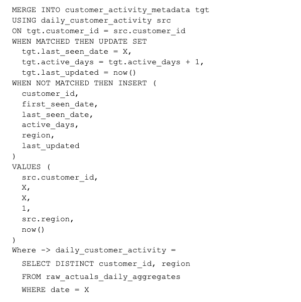
11. Additionally we would need a number of days since a customer is active on a platform for training the Forecast model. We will also create/maintain(optional in case another internal owns such dataset) a customer_activity_metadata table which is updated daily after updating the raw_actuals_daily_aggregates. [refer Appendix for the SQL]

Storage and compute requirements (BoE):

1. Input scan size: 10M customer x 500 SKUs x 20% (active SKUs) = 1B rows/day with ~100 bytes = 60–70Gb (compressed parquet)
2. raw_actuals_facts_daily : 1B rows X 70 bytes/row = 70GB/day
3. Raw_actuals_daily_aggregates : 10M x 30 (categories) x 50 bytes ~= 15Gb/day
4. Spark cluster sizing: Roughly 200–250GB I/O is expected in one cluster, with scoping of 1 hr max runtime we need: 40–60 cores assuming each core processes about ~150 Mb/min.

8.3 Feature Engineering Layer

We will produce 4 main features as defined below within a single spark job preferably :

1. Load raw_actuals_daily_aggregates from the previous step.
2. Compute rolling windows : last_3d_revenue, last_7d_revenue, last_30d_revenue, prev_30d_revenue, prev_7d_revenue for key (date, customer_id, category_id, canonical_category, region). Table: rolling_sales_features
3. Compute velocity : use the formula defined below in the Algorithms/logic section.
4. Compute trend_strength: use the formula defined below in the Algorithms/logic section.
5. Join calendar features : use the calendar_features table (date, region, is_holiday, holiday_name)

We attach day_of_week, is_weekend, is_holiday, days_to_holiday as columns

6. Write to feature tables. Table: market_dynamics_features_combined (all features combined)

7. Category_prior will be a separate Monthly job, calculated and kept to a separate table: category_prior_features. (Refer to Algorithms/logic section for formula)

8. All feature tables are located in s3 under s3://feature_store/v1/<table_name_as_path>

Storage and compute requirements (BoE):

1. Calendar table joins will be broadcast joins : 365 days x few regions
2. Input is about : 300M rows/day with window span of up to 30 days for few features.
3. Total daily output: 300M rows x ~90 bytes (combined all features) ~= 27Gb/day
4. Spark cluster sizing: shuffling overhead of windowed aggregations 15Gb/day X 30 day windows ~= 450 GB. (*need to validate with real execution). Roughly it would need 80–120 cores.

8.4 Forecast Model Training layer

Triggered by Airflow after feature Engineering DAG is successfully completed. Functionality will be implemented with Ray distributed training jobs on Kubernetes cluster(recommended to be managed on EKS or equivalent). MLFlow will be used for model registry.

Each Ray worker handles 1 customer 1 time series to train 1 model. The Ray Task Graph will be defined as :

Storage and compute requirements (BoE):

1. Customers trained: 10M (in worst case)
2. Avg training time/model : 6–8 sec
3. Total compute : (10 x 6)/3600 M hrs / 2 hrs [SLA] ~= 10K ray workers
4. Per ray worker ~= 1vCPU, 2 GB RAM. Physical compute needed = 10k vCPUs and 20TB RAM. Note: Compute needs are for 2–4 hrs in a quarter.
5. Avg trained model size = 100–200kb , Total storage needs = 200 x 10M KB ~= 2TB/day. We should be retaining only champion models for the long-term so this storage does not add over the time.

Training LightGBM or cohort models

The LightGBM model will be trained as a cohort-level supervised regression model using aggregated customer–category–region training rows derived from the feature store (velocity, trend_strength, calendar features, priors, and recent aggregates). The label is defined as realized revenue (or revenue share) over a fixed lookahead window (e.g., next 14 or 30 days) computed from raw_actuals_daily_aggregates.

Training data is stratified by canonical_category and lifecycle segment to ensure balanced representation and reduce bias toward high-volume cohorts. The model is retrained on a monthly cadence using 2–3 years of historical data and validated via temporal holdout and rolling backtests (MAPE, RMSE, bias). (Note: This will have similar DAG as Ranking weight Training model)

How do we manage MLflow for this scale of model tracking and metrics logging ?

MLflow will be deployed in a regional/country based cellular architecture. It is preferred to go with a Sagemaker Managed MLFlow setup from AWS for automatic scaling, patching and audit trails. Considering we will have millions of records generated after every full round of training every quarter. Considering the RDS data store for MLFlow does choke in terms of performance with a large number of records, we need the capability to purge older records from MLflow and move it to S3+ Andes for auditability. That leaves us with two options :

1. Use Managed MLflow with AuroraV2 serverless: for purges we will use a standalone job that uses mlflow.delete_run (rate limited to be < 200 deletes/sec per MLflow server) followed by mlflow.gc() call.
2. Use Self hosted MLflow (on ECS) and own AuroraV2 serverless: for purges we can delete records from DB directly although its slightly complex owing to relation data tables.

Considering this is once/twice a year activity, either of the two options can work. This is still a two way door decision but requires some additional effort in switching from one to another. With option 1, rough estimate is 6–8 days for cleaning up 50M runs on 1–2 t3.small instance(s) with nightly pauses during scheduled training runs.

For reads like where we need the champion model per customer MLFlow just can’t handle the reads. We will have to set up a cache in front of it only to store champion model versions.

If this doesn’t scale up, we will upgrade MEDS(discussed in next section) for our needs.

8.5. Ranking Weight Training Layer (Linear Regression Model)

The ranking weight training layer learns optimal weights for combining multiple predictive signals : short-term velocity, market trend strength, forecasted revenue, and category priors into a single scoring function used for category ranking. Training will be performed quarterly or monthly using a large, high-quality sample of customers with 2–3 yrs or longer historical coverage to capture stable, structural relationships between features and future sales outcomes. We will limit the training data set size with recommendations from core ML teams, for the purpose of this doc we will limit at 50k-100k customers. Supervised learning will be configured for a configurable 14-day look-back realised revenue share label, providing a balanced tradeoff between signal stability and responsiveness.

Score = w1 velocity + w2 trend + w3 forecast + w4 prior.

High level steps will be defined as below:

1. The training dataset consists of customers with a minimum of 2 years of historical data, limited to a set of 50–100k customers and stratified by representative and active canonical category to ensure coverage. Skewed or larger datasets will increase compute cost without proportional performance gains.
2. Time slicing on data of each such customer into T0 -> cold, T1-> growing, T2 -> mature. i.e. the same customer generates training examples for all 3 segments.
3. For each segment in parallel (dataset assembly per segment)

1. Fetch features for the scoring function: Input: velocity, trend, prior, forecast (market_dynamics_features_combined , forecasted_revenue, category_prior tables)

2. Compute Label: actual_next_14d_revenue_share calculated from raw_actuals_daily_aggregates.

3. Emits structured training rows (stored in s3://ranking-training/v1/[cold || growing || mature]) for regression model training.

4. Train linear regression model.

5. Offline validation : Rolling Backtest (refer to Model validation logic in Algorithms / Logic section)

6. Log the Model, its weight coefficients and metrics.

7. Compare the Production model with this challenger model. If Model validation logic succeeds, promote to “Staging” else retain champion.

8. Notify the Model Evaluation and Deployment Service (MEDS) (defined in later sections)

4. Training data Schema : event_date, customer_id, category_id, short_term_velocity, trend_strength, forecasted_revenue,category_prior, label_revenue_share_14d, segment, region, ingestion_ts.

5. Output: weight coefficients, model metrics and Model artifacts.

Pseudo code (generated)**

Storage and compute requirements (BoE):

1. Total record count = 100k customers x 30 categories x 730 days ~= 2 billion records (not all records are needed, this is only an upper bound)
2. Effective training rows ~= 20–50M (hand waving it here)
3. Data set size ~= 4–8 GB
4. Infra : small CPU batch job < 15mins (*if training data preparation is kept out of scope)
5. Model artefacts + MLFlow metadata = < 5 MB.

8.6 Model Registry & Governance

Until now models were only staged and not used to score any real customer. We define a control plane service called Model Evaluation and Deployment Service (a.k.a MEDS). MEDS will operate as a platform for A/B experimentation, traffic routing decisions, performance evaluation and model promotion.

• LR model training Airflow DAGs will use SnsPublishOperator or SNS webhook to trigger notification to which MEDS will be subscribed to via a SQS queue.
• MEDS writes the weight coefficients extracted from MLFlow data for the challenger model and updates the ranking_model_weights DB.
• It will then start recording A/B testing progress for the staging model(s) for 3 days (configurable).
• Nightly scoring jobs will use a deterministic hash based bucketing on (customer_id + model_segment + experiment_salt) assigning first N buckets to target N% of offline scoring traffic. This is a cheaper approach without storing per tenant state and can be extended for multi-challenger experiments as well by assigning disjoint bucket ranges to each challenger. (read comparisons in Appendix)
• MEDS tracks and monitors :

Rank churn rate (rank movements day over day)

% categories with large rank jumps i.e >2 or >3 position jumps.

Rank agreement vs prior day [similarity] (ranking looks similar to yesterday’s unless a real sales signal changed)

Distribution drift vs champion.

• MEDS on realisation and validation of results promotes a challenger model to “Production” or alerts the operations team with ticketing.
• Alternatives like Statsig or Eppo also enable A/B testing but they are purposed for online traffic. Sagemaker Model monitor is considerable for batch transform jobs but that duplicates the recommended Ray + Kubernetes infra. It does seem to route traffic per request but won’t be able to produce stable tenant-to-model mapping.
• Why is tenant based determinism important? If a tenant gets a different model based on scoring on consecutive days, they see ranking jumps and lose trust in the offering.

How do we do drift detection for the Linear regression models?

This needs more thought process on how do we automate a job that can extract a stratified sampled set by segment Cold, Growing & Mature. Mostly it should be a spark job that runs weekly and computes NDCG@5, Top-k Revenue capture, feature distribution drift (velocity, trend, forecast inputs) and stores the state in another trace table. Section 9 has some insights on alarming criteria which will be done from the spark job.

How does the system submit an async retraining request?

Drift detection publishes retraining signals (directly and/or via alarm action on the aggregate data points) to a decoupled queue based on appropriate priority, which are consumed by a scheduled orchestration DAG that performs priority-based, batched async retraining.This event-driven design will maintain controlled throughput and batching Ray jobs deterministically while keeping retraining loosely coupled with Drift detection logic. SQS-FIFO should be feasible in this case for the priority queue with lesser infra overhead as with Kafka.

8.7. Scoring & Precompute Layer

Precomputes top category rankings and forecast time series for all *enabled customers in batch mode to enable low-latency dashboard rendering and deterministic A/B evaluation.

Pipeline is orchestrated using Airflow nightly on Ray cluster. It consumes the latest feature dataset, the most recently published forecast models, and the ranking model weights, with a conditional switch between champion and optional staging versions based on experiment configurations, ensuring controlled rollout and reproducible inference.

Ray scoring cluster will load features, weights based on experiment config for a customer, compute scores, rank categories, detect drift to publish drift metric or alarm directly and then write results to DB. (for storage details see BoE below for this section)

• Table: customer_top_categories : stores top categories for user with customer_id and horizon#created_ts (rounded to date) as primary and secondary keys with other fields as top-categories (List<category_id>) , score-blob (binary) , forecasted_revenue, confidence_level, generated_ts, ttl_epoch. (ttl=120 hrs/ 5 days)
• Table: customer_category_forecasts : stores forecasts all horizons with primary key as combination of customer_id, category_id#date. Other fields include horizon_days, forecast_blob(Binary), compression(string, protobuf+ztsd), model_version, created_ts, ttl_epoch (now + 120 hrs), confidence_level.
• Table: customer_forecast_trace : focused to serve Forecast vs Actual historical trace (no TTL, long retention) view for the customer and drift detection metric storage. We will support paginated back date scrollable lookups on the forecast graph. Schema: customer_id, category_id#date, date, actual_val, forecasts_t1_val (number, T-1 for T), model_version, created_ts. (refer to section 10.3 for the additional set of metrics that will be stored in this table e.g MAPE)
• Additionally, Ray job will also write these data sets to S3 for long term retention, training, drift detection, auditing and analytics requirements.

*enabled customer: customers who have activated forecasting features. (can bring in activity_metadata as well, for e.g. if customer has not logged into the system for over 60 business days, async triggers can be built but keeping it out of scope)

Storage and compute requirements (BoE plus comparison of approaches):

For customer_category_forecasts:

1. To support is 1 year i.e 365 days of forecast datapoints for 10M customers (upper bound) ~= 10M x 5 (top 5 only) x 365 = 18B rows/night.

Approach 1: write per data point records in db

If 4 hrs is the completion time for the nightly scoring job, then expected sustained write rate is ~= 18B/15k seconds ~= 1.2 Million writes/sec.

(-) This is feasible but very expensive operationally as well as AWS bill wise. Batched writing will push job time by minutes/hours with recurring retries due to timeouts.

Approach 2 : storing all data points as blobs in a single record in Dynamodb.

Considering, if we can store 90 days data points or entire 365 data points in a single row.

365 data points ~= 8 bytes x 365 x 3 arrays ~= 12 kb

Total WCU needed per row for 365 days ~= 12

Compared to daily rows (1.3 M WCU/sec), we would need 40k WCU/sec with 365 day blobs, although it still costs $950/day only in writes.

Approach 3: Only keep metadata in DB and datapoint blob in S3 for 90 and 365 days horizons.

(+) cheaper alternative

(-) S3 adds a read overhead latency of 100–200ms P50.

Approach 4: Keeping Metadata in DB, datapoints blobs in S3 and Redis cache.

(+) faster than all alternatives

(-) Cost-wise slightly higher than the Compressed DynamoDb storage solution.

(-) More complicated with more components to handle operationally. Redis cluster needs to handle sustained writes (200Gb in minutes) and would be ~10–12 nodes cluster running 24x7 (costs roughly $8–10K/month for r6.4xlarge).

(-) High read volume is not expected considering a customer would fetch forecasts 4–6 times a day. So it doesn’t make sense to have a full blown Redis cluster for storing precomputed data.

[Recommended] Approach 5: Using data compression for the forecast blob storage in Dynamodb

We know that Prophet or SARIMA timeseries forecasts usually produce “smooth” curves with mathematical correlation between adjacent days. This enables compression with solutions like delta encoding and quantization that cuts size by 75–90%. A quick search on Protobuf + ztsd could effectively reduce write costs to ~$150–200/day.

(-) latency tax of 5–10 ms at server end to extract data blob before returning processed response to customer window.

8.8. Durable data storage, Caching and Request Serving

• Feature & training data sets are stored in S3 as iceberg tables registered on glue catalog.
• Model registry is stored on MLFlow
• Scoring Output and Forecast TimeSeries is stored on DynamodDb (managed and horizontally scalable database with five nines of availability) with a read through cache like DAX or with Redis. We expect 5–10 reads within a day per customer, which is workable with a small sized cache in front of DB although optional.

8.8.1. APIs / Interfaces

• GET /v1/customers/{id}/top-categories?timeframe=week | month | year
• GET /v1/customers/{id}/forecast/{category_id}?timeframe=week | month | year

8.8.2 Optional Cache Keys for Redis or in-memory Guava cache:

• top_categories:{customer_id}:{timeframe}:{generation_vs}
• forecasts_ts:{customer_id}:{category_id}:{generation_vs}
• top_categories:current:{customer_id}:{timeframe} [pointer for atomic updates]
• forecast_ts:current:{customer_id}:{category_id} [pointer for atomic updates]

9. Algorithms / Logic

This section summarises all algorithms and logic used in above sections for clarity. (attaching the image as it super hard to convert the formulas for the google doc to here)

10. Operational Considerations

10.1. Deployment:

• [CI/CD pipelines with AWS CDK or suitable infra used within Intuit]

10.2. Monitoring & Logging:

We will use AWS managed services for Prometheus (AMP) and Grafana (AMG) for horizontally scalable monitoring stack as a cheaper and vendor neutral alternative to CloudWatch monitoring. Prometheus is recommended for Kubernetes because it uses Kubernetes service discovery to automatically find pods via labels.

10.2.1 Model Performance Monitoring

1. Forecast Models: MAPE, RMSE, Bias, Drift metrics
2. Ranking Models: NDCG@K, TopK Revenue capture, CTR lift / Customer engagement (online A/B)

10.2.2. Online Serving: (Four Golden rules for core metrics)

• API Latency
• Number of Requests
• Cache Hit ratio (optional)
• Error Rate
• Saturation: CPU-util, Memory-util, I/O

10.2.3 Data Quality Monitoring :

• Zero sales anomalies
• Category skew
• Missing data rate

10.2.4. Training and Ranking pipeline Monitoring:

• DAG success rate (alarm on failure)
• Training Job runtime
• Scoring job latency
• Saturation : CPU usage /Memory usage

10.3. Alerts & Threshold

Notification action on alerts will be Ticketing and based on its severity (Critical) PagerDuty would notify on-calls.

Forecast and Ranking model Alerts:

Pipeline health alerts:

• DAG execution failure, training time and scoring delay beyond thresholds leads to tickets.

Service Layer alerts :

• API latency > 200ms P99 for X mins , error rate > 0.5% for X mins
• Burn rate: cache hit rate < 97% for 15 mins (warning) , cache hit rate < 95% for 5 mins and DB RPS increases (critical)

10.4. Performance (SLOs) — Monthly:

• API Latency (<200ms @P95 and < 500ms @P99)
• Cache Hit rate: >= 98%
• Availability of service 99.9%
• Data freshness : velocity, Trend/prior, Forecast <=24 hrs
• Ranking correctness: < 0.1% invalid responses , 0 tolerance for malformed rankings
• Rank volatility : ≤ Y% of categories change rank by >2 positions day-over-day, unless velocity spike exists.

11. Security & Compliance

11.1. Security requirements:

• IAM based authentication and authorisation for cross team data access (least privilege principle to be followed)
• We will use Lake formation for fine grained access control to datasets (LF-tags or ABAC)
• Private VPC, security groups + NACLs for compute cluster
• Audit logs for accesses: model registry, scoring APIs , training jobs. (Use S3 for immutable storage)
• API gateway + Oauth2/JWT (this is an assumption, we will use existing auth controls in QB)
• Model versioning only through MLFlow
• Model artefacts to be signed : use KMS asymmetric key and SHA-256 hash of the model.onnx file
• Encryption at rest (S3 : SSE-KMS, DB — KMS encrypted data, Redis cache: encrypted snapshots) and in-transit (TLS 1.2+)

11.2. Compliance (GDPR/CCPA & PII)

• Right to erasure : Remove customer data within 30 days after cancellation. Need separate cron jobs for clean up and configuration flags to disable processing a cancelled customerId. (Keeping out of scope of this doc but this is mandatory)
• Customer identifiers to be pseudonymized and no PII to be stored
• Anonymisation for ‘Global Trends/priors’ (Rankings are potentially inferential of competition):

Step 1: we enforce K-anonymity i.e generate cohort signals only if there are at least k distinct customers in a peer group (category + region).

Step 2: Progressive generalisation i.e we go global if k-anonymity is not met in step 1. (Category, city) — -> (category, country) — -> (category, global)

This should be enough considering we have a LR model that provides 3 sets of weights based on tenants age. So the risk is very low in our case.

• No logging of customer_ids, revenue, sales info to logs: implement Log Redaction at collector level using ADOT Redaction processors. All customer data is marked or hashed before it leaves EKS cluster(no PII in log)

12. Testing Strategy

12.1. Unit Tests :

• Validate Spark transformations (null handling, dedupe, UTC normalization)
• Feature calculations (rolling windows, velocity, trend formulas)
• Model training logic (segment splits, label correctness)
• Protobuf serialization/deserialization of forecast blobs
• Compression integrity (round-trip tests: compress → decompress → compare)

12.2. Data Quality tests:

• Schema validation for all tables (Glue/Iceberg/DynamoDB items)
• Null, range, and monotonicity checks (revenue ≥ 0, valid dates)
• Distribution drift checks on features (velocity, forecast, prior)
• Row count reconciliation (input vs output per DAG stage)

12.3. Offline mode Evaluation

• Temporal holdout validation (no leakage in time series)
• Rolling backtests (T+1 accuracy vs actual)
• Segment-wise metrics (cold/growing/mature)
• Weight Coefficient sanity checks (sign, magnitude stability)

12.4. Integration Testing (Pipeline DAG)

• End-to-end run on sampled dataset (e.g., 1K customers)
• Validate handoffs: Feature Store → Ray → DynamoDB
• Ensure TTL fields, keys, and blobs are written correctly
• Idempotency tests (re-run DAG should not corrupt state)

12.5. Performance & Load Testing

• Simulate nightly scale (10M customers, batched Ray jobs)
• Measure forecast generation time vs 4-hour SLA
• DynamoDB write throughput tests (WCU, throttling, retries)
• Redis/Dynamo read latency under peak load

12.6. Failure & Resilience Testing

• Inject worker failures in Ray (retry validation)
• Partial DB write failures (batch retry correctness)
• Backpressure handling and checkpoint recovery

12.7. UI & Trace Validation

• Forecast vs actual graph correctness (T-90 vs T+1 trace)
• Blob decompression latency checks
• Consistency between trace table and forecast table

12.8. Monitoring & Regression Safeguards

• Automated daily metric thresholds (MAPE, drift, latency)
• Canary runs on small cohort before full rollout
• Model version rollback testing via MLflow + MEDS

13. Alternatives Considered

13.1. Compute options comparison

Ray cluster vs Sagemaker:

Ray+ kubernetes is better suited for massive, fine-grained workloads (per customer time series), offering low task startup overhead, high resource utilization, cost efficiency with spot instances (EKS), and strong fault isolation without vendor lock-in, though it requires more engineering effort and complex setup. Ray offers orchestrating custom DAGs, caching, batching and DB writes in one runtime.

In contrast SageMaker Pipelines is a fully managed, easy-to-use solution with built-in ML lifecycle tools and faster deployment, but it can be less efficient and more costly (managed instances) at large task scale due to higher startup overhead, coarse scheduling, and increased dependency on one cloud vendor.

We recommend “Ray on kubernetes” as it provides a scalable, long term solution for trivially parallel, requiring fine grained distributed task execution at massive scale (~10 M series per night) while offering better cost efficiency in the long term.

13.2. Storage options comparison

DynamoDb vs Aurora(Postgres)

• Bursty write pattern of up to 15ks writes/sec nightly: Aurora would face write contention and scaling limits at 2 am in night.
• TTL support for auto-expiry is not present in any of the managed postgres DB solutions (checked on Aurora offering from AWS).
• Storage needs range between 1–2 TB given the flexibility on TTLs. (Forecast table: 50M x 5 days x 4kb ~= 1 TB, Trace table: 3.5 Gb/day).
• Given that there are no relational joins needed with horizontal partitioning eliminating hot shard risks, we will go with Dynamodb for its serverless scaling for high write throughput. It is scalable to support even 10 top categories and requires no sharding as customers grow from 10M to 100M.

13.3 Monitoring stack comparison

Prometheus Vs Cloudwatch

14. Future works

• Using category-level forecasting and proportional SKU allocation for cheaper and scalable SKU-level forecasts in the UX where customers can update the proportion to better observe the variations in future and make reports out of it.
• Allow customers to update the forecast with user provided numbers to reflect into reporting (WHAT-IF-SCENARIO with manual targets).

15. Appendix

15.2. SQL code snippets:

15.3 References:

1. https://docs.aws.amazon.com/forecast/latest/dg/aws-forecast-choosing-recipes.html
2. https://docs.aws.amazon.com/aws-supply-chain/latest/userguide/forecast-algorithims.html []
3. https://www.uber.com/en-IN/blog/ubers-journey-to-ray-on-kubernetes-ray-setup/
4. https://www.anyscale.com/blog/training-one-million-machine-learning-models-in-record-time-with-ray
5. https://www.alibabacloud.com/blog/602313
6. https://medium.com/walmartglobaltech/optimizing-api-performance-with-zstd-compression-and-protocol-buffers-571ad30f4893