Measure of Central Tendency & Dispersion

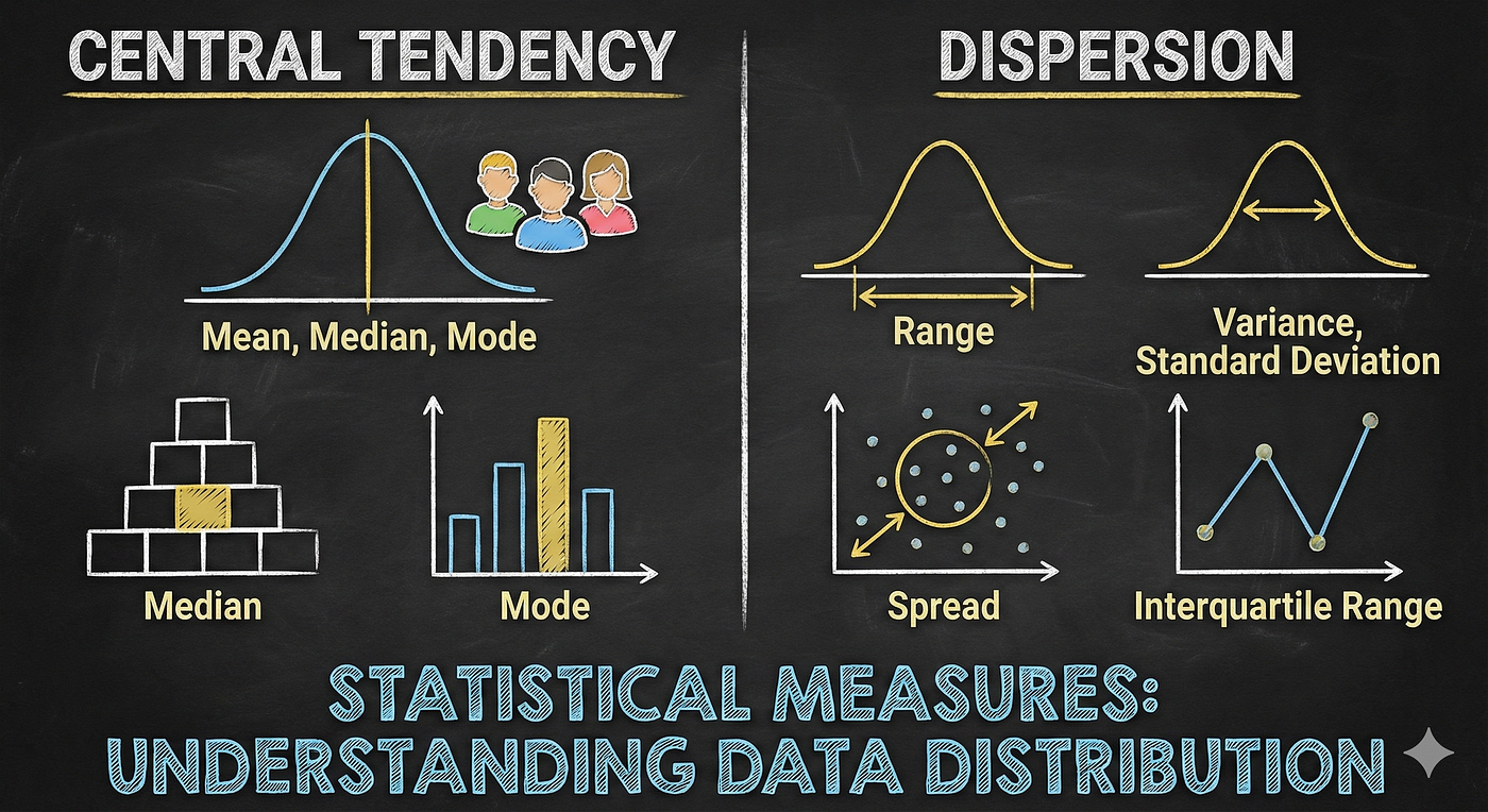
Measure of Central Tendency & Dispersion

Measures of Central Tendency

A measure of central tendency is a statistical measure that represents a typical or central value for a dataset. It provides a summary of the data by identifying a single value that is most representative of the entire set.

1. Mean (Average): The mean is the sum of all values in the dataset divided by the total number of values. Note: It is highly prone to outliers, so it should only be used when the data is symmetrically distributed without extreme values.

• Example: The mean age of a team of 5 people (22, 24, 25, 28, and 31) is calculated as (22 + 24 + 25 + 28 + 31) / 5 = 26 years old.

Mean (Average)

2. Median: The median is the exact middle value in a dataset when the data is arranged in numerical order. If there is an even number of data points, the median is the average of the two middle values. Note: It is highly resistant to outliers because extreme values sit at the very start or end of the sorted list and don’t pull the middle value away.

• Example: In a sorted list of five salaries ($40k, $45k, $50k, $55k, $1 Million), the median is $50k, which is a much more accurate reflection of the “typical” salary than the mean would be.

Median

3. Mode The mode is the value that appears most frequently in the dataset. It is specifically useful for categorical data or discrete numerical data where you want to know the most common occurrence.

• Example: If a shoe store’s sales records show sizes 7, 8, 8, 8, 9, and 10 were sold today, the mode is size 8.

4. Weighted Mean The weighted mean is the sum of the products of each value and its assigned weight, divided by the total sum of the weights. It is used when the values in a dataset have different levels of importance or frequency.

• Example: Calculating a student’s final grade where the final exam is worth 50% (weight 0.5), the midterm is 30% (weight 0.3), and homework is 20% (weight 0.2).

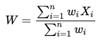
Weighted Mean

5. Trimmed Mean A trimmed mean is calculated by sorting the dataset, removing a certain percentage of the smallest and largest values (the trimming percentage), and then taking the mean of the remaining values. Note: This is an excellent way to automatically remove outliers. Box plots are often used first to identify if trimming is necessary.

• Example: A 10% trimmed mean of 20 test scores involves dropping the 2 lowest and 2 highest scores, and then averaging the remaining 16 scores.

Trimmed Mean

Measures of Dispersion

A measure of dispersion (also known as variability) describes the spread of a dataset. It provides critical information about how closely or loosely the data points are distributed around the central tendency. It is used becuase if two dataset have same mean don’t mean both dataset have same dispersion.

1. Range: The range is simply the difference between the maximum and minimum values in the dataset. It is the simplest measure of dispersion, easy to calculate, but extremely sensitive to outliers.

• Example: If the daily temperatures for a week are 15°C, 18°C, 20°C, and 35°C, the range is 20°C (35–15).

Range

2. Variance: The variance is the average of the squared differences between each data point and the mean. It measures the average distance of each point from the mean. Note: We square the differences to prevent positive and negative values from canceling each other out. Because of the squaring, variance is highly prone to outliers (an outlier’s distance gets squared, making it exponentially larger). The unit of variance is also squared.

• Example: If calculating the variance of people’s heights measured in meters, the variance unit would be “square meters,” which isn’t intuitively easy to visualize.

Variance

Why is n-1 used in Sample Variance? When we calculate the variance of a sample to estimate a population, dividing by n (the total number) consistently underestimates the true population variance. Dividing by n-1 (known as Bessel’s correction) slightly increases the result, providing a much more accurate, unbiased estimate of the broader population.

3. Mean Absolute Deviation (MAD): It is similar to variance, but instead of squaring the differences, we use the modulus (absolute value) to prevent negative and positive distances from canceling out. Note: Because we don’t square the numbers, it is not severely prone to outliers like variance is, and the unit remains the exact same as your original data. However, it is used less frequently in advanced statistics because absolute values are harder to use in algebraic equations.

• Example: If the average test score is 80, and the MAD is 5, it means that on average, a student’s score deviates by exactly 5 points from the mean.

Mean Absolute Deviation

4. Standard Deviation: The standard deviation is the square root of the variance. It is the most widely used measure of dispersion. Note: Since the unit of variance is squared, taking the square root returns the metric back to the original unit of your data, making it easy to compare directly with the mean i.e. unit remains the exact same as your original data. It is mostly used in place of vairance becuase of same unit.

• Example: If the variance of the heights is 0.04 square meters, the standard deviation is 0.2 meters, meaning heights typically vary by about 0.2 meters from the average.

Standard Deviation

Q. Train A has average late time of 10 hours and standard deviation late time
of 2 hours. while Train B has average late time of 10 hours and standard 
deviation late time of 6 hours. I only afford to be 1 hour late? then which 
train should i travel with?

Answer. You should travel with Train B.While both trains are expected to be 10 
hours late on average, Train B has a much higher statistical variation 
(standard deviation). This means Train B's actual arrival times fluctuate 
wildly, making it the only train with a realistic chance of running 
significantly ahead of its terrible average schedule and arriving less 
than 1 hour late.

5. Interquartile Range (IQR):

Quantiles

Quantiles are statistical measures used to divide a set of numerical data into equal-sized groups, with each group containing an equal number of observations. They are important measures of dispersion and can be used to understand the distribution of data, summarize it, compare different datasets, and identify outliers.

There are several types of quantiles used in statistical analysis, including:

• Quartiles: Divide the data into 4 equal parts: Q1 (25th percentile), Q2 (50th percentile or median), and Q3 (75th percentile).
• Quintiles: Divide the data into 5 equal parts: Q1 (20th percentile), Q2 (40th percentile), Q3 (60th percentile), and Q4 (80th percentile).
• Deciles: Divide the data into 10 equal parts: D1 (10th percentile), D2 (20th percentile), …, D9 (90th percentile).
• Percentiles: Divide the data into 100 equal parts: P1 (1st percentile), P2 (2nd percentile), …, P99 (99th percentile).

Things to remember while calculating these measures:

1. The data must be sorted from lowest to highest.
2. You are essentially finding the location of an observation at a certain percentage point.
3. The calculated quantile value might not be an actual number present in your dataset (it may fall between two numbers).
4. All other tiles (Quartiles, Deciles, etc.) can be easily derived directly from Percentiles.

Percentiles

A percentile is a statistical measure that represents the percentage of observations in a dataset that fall below a particular value. For example, if you score at the 75th percentile on a test, it means your score was higher than 75% of the people who took it.

Formula to calculate the value at a Specific Percentile or location of a percentile in your dataset:

Formula to calculate the percentile value

Example: Find the 75th percentile score from the given data: 78, 82, 84, 88, 91, 93, 94, 96, 98, 99.

1. Sort the data in ascending order: 78, 82, 84, 88, 91, 93, 94, 96, 98, 99.
2. **Calculate the Location (PL): **PL = 75 (10+1)/100 = (7511)/100 = 33/4 = 8.25*
3. Interpolate the final value: Since the location is 8.25, the value falls between the 8th data point (96) and the 9th data point (98).
4. 75th percentile = 8th value + 0.25 (9th value — 8th value) = 96 + 0.25 (98–96) = 96 + 0.5 = 96.5 Answer

Formula to calculate the Percentile of a Specific Value:

Formula to calculate the Percentile of a value

Example: Find the percentile of the number 88 from the given data: 78, 82, 84, 88, 91, 93, 94, 96, 98, 99.

1. Sort the data: 78, 82, 84, 88, 91, 93, 94, 96, 98, 99.
2. Identify variables: There are three numbers below 88 (X = 3), one number equal to 88 (Y = 1), and ten numbers total (N = 10).
3. Percentile of number 88 = The number 88 sits at the 35th percentile.

5-Number Summary

The 5-Number Summary is a descriptive statistic that provides a quick, comprehensive overview of a dataset. It consists of five values that divide the dataset into four equal parts (quartiles). The five-number summary includes:

1. Minimum value: The absolute smallest value in the dataset.
2. First quartile (Q1): The 25th percentile; the value that separates the lowest 25% of the data from the rest.
3. Median (Q2): The 50th percentile; the exact middle value separating the lowest 50% from the highest 50%.
4. Third quartile (Q3): The 75th percentile; the value that separates the lowest 75% of the data from the highest 25%.
5. Maximum value: The absolute largest value in the dataset.

5-Number Summary

Note: In Python, you can quickly generate this using the describe() function in the Pandas library.

Interquartile Range (IQR)

The IQR is a measure of variability based directly on the 5-number summary. Specifically, the IQR represents the middle 50% of your data and is defined as the difference between the third quartile (Q3) and the first quartile (Q1). Formula: IQR = Q3 — Q1

6. Coefficient of Variation (CV): The CV is a statistical measure that expresses the amount of variability in a dataset (Coefficient of Variation) relative to the mean. It is a dimensionless quantity (having no units) expressed as a percentage. It is incredibly useful when you need to compare the spread of two different columns of data that are on completely different scales.

• Example: Comparing the price volatility of a $10 stock with a $500 stock. A standard deviation of $1 is huge for the $10 stock (CV = 10%) but virtually unnoticeable for the $500 stock (CV = 0.2%).

Coefficient of Variation

7. Lorenz Curve: A graphical method used to visualize inequality or dispersion, often in income distribution.

Types of Dispersion Measures:

• Absolute Measures:
• Relative Measures (Coefficients):

Commonly Used Relative Measures:

• Coefficient of Variation (CV): Standard Deviation divided by the Mean, often expressed as a percentage.
• Coefficient of Range:
• Coefficient of Quartile Deviation: