Artificial Neural Network Model to Solve the Inverse Kinematics of a 5-DOF Manipulator

Background

The motion of a robot manipulator can be described by the kinetic chain, which is an assembly of rigid bodies connected with joints. By attaching coordinate frames to each of the joints, we can derive transformation matrices that describe the relationship (translation and rotation) between two adjacent frames of the manipulator. Multiplying all the attained transformation matrices in series, we get the final transformation matrix that describes the position and orientation of the end-effector with respect to the base frame. This process of calculating the position and orientation given the joint parameters is called forward kinematics, or direct kinematics.

Inverse kinematics is the reverse process of computing the joint parameters when the position and orientation of the end-effector are specified. However, unlike forward kinematics, the analytical solution, or closed-form solution of inverse kinematics can be challenging to derive, even more so as the manipulator takes a more complex form with higher degrees of freedom. Furthermore, with recent robotic applications continually emphasizing fast computation speed, the need for a simpler, quicker method to solve inverse kinematics arises. Although difficult to obtain, closed-form inverse kinematics solutions always exist for a manipulator made of rigid links. But imagine a robot manipulator made of compliant structures. Due to the flexibility of the entire structure that allows movement in infinite directions, it is no longer easy to derive the inverse kinematics solution. In such a case, data-driven approaches might be the only viable option.

In this article, a machine learning model was designed using the artificial neural network architecture to solve the inverse kinematics solution of a custom-built 5-DOF manipulator.

Dataset Generation

The dataset contains 100,000 artificially generated data points for a custom-made 5-DOF manipulator. Since the configuration of the coordinate frames for each of the joints in the manipulator is known, we can formulate the Denavit-Hartenberg parameter table, which allows us to derive the transformation matrix that describes the position and orientation of the end-effector with respect to the base link. This transformation matrix returns a 4x4 matrix whose components are all given as functions of the joint angles, q1, q2, q3, q4, q5.

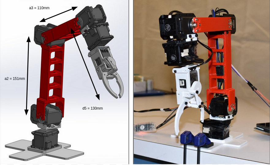
Figure 1. The robot manipulator with its link lengths and offset labeled.

Figure 2. The Denavit-Hartenberg parameter table and the transformation matrix.

Now that the we can model the position and orientation of the robot manipulator through the transformation matrix when all the joint angles are given, it is time to generate the data that will be used to train the machine learning model. After defining the lower and upper limits for each of the five joints, we use np.random.uniform to randomly generate 100,000 uniform data points within these lower and upper limits . This process is repeated for all five joints. Lastly, the randomly generated joint angle values are concatenated to form 100,000 possible combinations of q1~q5. It is then inserted into the transformation matrix to obtain the position (x, y, z) and orientation (R11, R12, R13, R21, R22, R23, R31, R32, R33) of the end-effector. These 12 terms will the input to the neural network, which will predict the joint angles q1, q2, q3, q4, q5.

In order to store the obtained values of the position and orientation from the transformation matrix given the joint angle inputs, a for loop iterates from 1 to 100,000 and stores each of the obtained values in a row in predefined order, which is inserted into a pandas dataFrame. Finally, we have a dataFrame with 100,000 datapoints and 17 columns. The dataframe is saved in .csv format and is read from another python script that preprocesses the data and trains the network.

The true beauty of this problem lies in the inexpensiveness of the data. The link lengths and link offsets can easily be defined through the 3D model of the robot. With this, we can then formulate the DH-parameter table, which is then used to form the transformation matrix. The entire process of calculating the forward kinematics is straightforward and once the joint angle combinations are specified, new data is easily generated. Since, the generated data follows a mathematical equation, no datapoints are invalid, which can also facilitate the training process.

Training the Neural Network

This problem is an example of multi-output regression, in which we are trying to obtain the joint angle values q1 ~ q5 through position(x, y, z) and orientation(R11, R12, R13, R21, R22, R23, R31, R32, R33) input.

First, the data generated data described earlier is loaded, and the features are separated from the label. After the features are separated from the labels, scikit-learn’s train_test_split is used to split and shuffle the training and testing data. Since the size of the dataset is large, only 5% of the total data is allocated for testing.

Next, the features are normalized. The mean of the training data is calculated, which is then subtracted from the original data, then divided by the standard deviation. This process is necessary for successful training, to ensure all the features are across similar scales. After this step, the data is prepared to be fed into the network for training!

The network’s architecture was created using keras’ sequential class. The network consists of 4 fully-connected hidden layers, all with 100 units, followed by ReLU as the activation function. The output layer has 5 units corresponding to each of the five joint angles. RMSprop was used as the optimizer with 0.01 learning rate, and mean squared error was selected as the loss function.

Figure 3. The architecture of the NN

Finally, after building the model, the training features and labels were fitted to the model with the following parameters: batch_size=24, epochs=1000, validation_data=[X_test, y_test], callbacks=[callback]. In order to avoid overfitting, EarlyStopping was used as a callback to monitor the validation loss, which is the mean_squared error on the test dataset. The minimum delta value was set at 0.05 with the patience value of 20 epochs.

Model Validation and Conclusion

The training was stopped after 34 epochs, obtaining the mean-squared-error or 0.2629 and 0.2411 for the training and testing datasets respectively. Comparing the loss values for the training and testing dataset, we can conclude that the model has not overfitted and in fact, generalized quite well to unseen data. Although the small difference in training and validation loss indicates that the model was somewhat successful in predicting the joint angles of the manipulator, we need to dive deep on the meaning of the mean-squared-error value of 0.2411. This roughly corresponds to being off by about 4 degrees for each joint angle. In an area of application that requires extreme accuracy such as robotic manipulation, this value is not negligible.

Figure 4. Training loss and validation loss of the trained neural network.

Despite the relatively large error considering the exactness demanded in the field of robotic manipulation, the fact that the model has performed equally as well on unseen data as with trained data suggests that a small fine touch could possibly decrease the error, so that data-driven methods could one day replace closed-form solutions to inverse kinematics. The following are some suggested areas of improvement.

• Improve the quality of generated data. Currently, the data was randomly, uniformly generated for each joint angle. This does not necessarily consider the uniformity in the combinations of the joint angles. By providing data that spans through all of the manipulator’s working space, this would expose the network to most possible scenarios.
• Implement tools like scikit-learn’s GridSearch for hyperparameter tuning. Experimenting between different choices of layer depth and width, activation function, optimizer, learning rate, batch size and many more will most likely lead to the discovery of a better suited network to the current data.