How to Scale Optuna Without Breaking Bayesian Optimization

Optuna is excellent for hyperparameter optimization, but the naive way to scale it can quietly undermine the very thing that makes Bayesian optimization valuable: coordinated, information-efficient search. Simply increasing n_jobs or n_threads is not the same as getting a better parallel Bayesian optimizer, and Optuna’s documentation treats parallel execution as an execution strategy rather than as a batch acquisition method in its own right.

The core issue is simple: most of Optuna’s default samplers, especially TPE, are fundamentally designed to propose one point at a time. If multiple workers request suggestions concurrently, they are not jointly choosing a batch of points that works well together; they are making several independent sequential-style decisions at once. That distinction sounds subtle, but it matters a lot in practice.

Why more threads are not enough

When people first try to scale Optuna, the obvious move is to increase n_jobs. That does increase throughput, but it does not automatically preserve the statistical efficiency of Bayesian optimization. With TPE, each worker samples based on the current trial history, but there is no true joint batch optimization over pending suggestions. In effect, parallel workers are not coordinating to cover different promising regions of the search space; they are each making local decisions using nearly the same information.

That becomes especially problematic when the objective has strong signal. If the sampler quickly identifies one promising region, multiple workers can collapse toward that region at the same time, producing duplicate or near-duplicate trials. Optuna users have repeatedly reported duplicate suggestions and reduced reproducibility in parallel TPE settings, which is exactly what should be expected from a sequential sampler being run concurrently without a batch-aware acquisition rule.

This is the irony of naive parallel Bayesian optimization: the more structure there is in the problem, the easier it is for uncoordinated workers to chase the same structure redundantly. Parallelism increases throughput, but without a batch policy it can reduce information gain per trial.

What TPE is actually doing

Under the hood, TPE does not build a global latent model of the objective in the same way that a Gaussian process does. Instead, it splits prior observations into “good” and “bad” sets and fits density estimators over the parameter values, then proposes new points by favoring regions where the ratio of those densities is high.[cite:11][cite:77] In Optuna, TPE operates over the search-space coordinates exposed through suggest_float, suggest_int, and suggest_categorical, which means it reasons directly over those parameter values rather than over an explicit semantic geometry of the problem.

That is perfectly reasonable for many hyperparameter optimization problems. If the task is to tune learning rate, weight decay, depth, or regularization, a density model over parameter values is often enough to work well. But it also means TPE does not have a notion of a jointly optimized batch, and it does not have a parameter analogous to “number of batches” or batch size in qEI. Setting n_jobs > 1 does not transform TPE into batch Bayesian optimization; it just runs multiple sequential proposals in parallel.

This is also why there is no TPE knob that corresponds to “make the batch search more thorough.” TPE has tuning parameters that affect its density estimates and sampling behavior, but not a true batch-size parameter that changes the underlying decision problem the way qEI does.

What real parallel BO looks like

If the goal is to preserve the value of Bayesian optimization while evaluating many trials at once, the right abstraction is a batch acquisition function. Instead of asking for one point repeatedly, a batch acquisition function chooses a set of points that is good collectively. That is a different optimization problem from simply asking a sequential sampler for several points at the same time.

Expected Improvement is one of the most widely used acquisition functions in Bayesian optimization because it cleanly balances exploitation and exploration. Its batch extension, qEI, asks a more relevant parallel question: what is the best set of q points to evaluate next, given uncertainty in the surrogate model and the interactions among pending candidates? That gives qEI a clean conceptual advantage over n_jobs-style parallelization of a sequential sampler.

This is the most important scaling lesson: increasing n_jobs makes the execution engine busier, but increasing q changes the optimization problem itself. In other words, n_jobs makes a sequential policy faster; qEI makes a parallel policy better.

A concrete experiment on ad embeddings

To make this less abstract, consider a real ad-quality modeling task referred to here as **chi-bad-ads**. The dataset maps each ad’s embedding to a human-labeled “badness” target, where higher values mean the ad is judged worse on average. The input is a dense embedding vector per creative, and the output is the average human label for that creative. The surrogate model is a Gaussian Process Regressor fit not on raw embeddings but on a 64-dimensional PCA projection of those embeddings, which keeps the optimization space continuous and tractable.

The target is transformed as well: the score is treated as log-normal, so the logarithm of the target is approximately Gaussian before fitting the GP. That matters because standard GP regression assumes Gaussian residual structure, and this transform makes the posterior and the resulting acquisition behavior more stable and interpretable.

In this setup, the GP is operating in a continuous latent space built from ad embeddings, with PCA reducing them to 64 dimensions. You can think of this as a “meaning space” for creatives: nearby points tend to correspond to ads with similar content and style. That matters for this experiment because qEI is choosing batches in a space where distance has semantic meaning, not just in a flat grid of IDs.

The experiment compares 4 settings:

• Optuna with default TPE sampler
• qEI with a batch size of 512.
• qEI with a batch size of 4,096.
• Random search with the same total trial budget.

The 512-batch setting is the practical regime. The 4,096-batch setting is more like an aggressive upper-bound regime: if the acquisition function can search over a much larger batch each round, how much better does it get? Random search provides the baseline.

Each iteration performs 4 evaluations in parallel. The experiment is repeated 12 times with different random seeds. The averageof the current “best so far” is shown below:

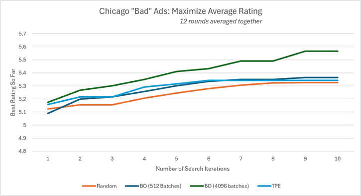
qEI (4096 batches) clearly dominates TPE for the same number of parallel workers

The first thing to notice is that the 512-batch qEI run beats or matches random search in every round after the first, usually by around 0.04 to 0.06 on the transformed target. That already shows the value of coordinated batch selection over unguided exploration.

The more interesting point is that the 4,096-batch qEI run is substantially better than the 512-batch and Optuna TPE runs. That gap is not an artifact of using more total trials; the total trial counts in the table are the same. The difference comes from the acquisition step being allowed to optimize over a much richer candidate batch each round.

That is exactly the kind of effect that naive n_jobs parallelization cannot reproduce. Increasing batch size in qEI changes the combinatorial decision being made: the optimizer can cover multiple promising regions of the latent space at once. Increasing n_jobs for a sequential sampler does not do that. It just makes the same one-point policy speak faster.

This is also why the embedding-based setup matters here, but only as supporting intuition rather than as the article’s main point. In this experiment, the GP is exploiting a continuous latent structure over ads, so better batch planning has a meaningful geometry to work with. In many standard HPO settings, the semantic interpretation is less important. The central lesson still survives: proper batch BO scales more intelligently than naive concurrency.

Using Optuna the right way

None of this means Optuna is the wrong tool. It means Optuna is best used as the orchestration layer, while true batch Bayesian optimization logic lives in the acquisition step. Optuna’s ask-and-tell interface is designed for exactly this kind of external control loop.

A standard ask-and-tell loop in Optuna looks like this:

study = optuna.create_study(direction="maximize")
for _ in range(n_trials):
    trial = study.ask()
    x = trial.suggest_float("x", -10, 10)
    y = objective(x)
    study.tell(trial, y)

To make this batch-aware, the pattern changes slightly. Instead of letting Optuna’s internal sampler decide the next suggestions, the next batch is chosen by an external GP + qEI routine provided by the quantecarlo library, and Optuna is used purely to track trials and outcomes.

# pip install quantecarlo

import optuna
from concurrent.futures import ThreadPoolExecutor
from optuna.trial import TrialState
from quantecarlo import DimSpec, qEISampler

# Search space: names and bounds must match suggest_* calls.
search_space = [
    DimSpec(name="x", type="float", low=-5.0, high=5.0),
    DimSpec(name="y", type="float", low=-5.0, high=5.0),
]

Q = 4               # batch size and number of parallel workers
N_STARTUP = 8       # random warm-up trials before GP-based qEI
N_ITERATIONS = 10   # total trials = N_ITERATIONS * Q

def objective(trial: optuna.Trial) -> float:
    x = trial.suggest_float("x", -5.0, 5.0)
    y = trial.suggest_float("y", -5.0, 5.0)
    return (x - 1.3) ** 2 + (y + 0.7) ** 2   # minimum at (1.3, -0.7)

sampler = qEISampler(
    search_space=search_space,
    q=Q,
    n_startup_trials=N_STARTUP,
)

study = optuna.create_study(direction="minimize", sampler=sampler)
optuna.logging.set_verbosity(optuna.logging.WARNING)

with ThreadPoolExecutor(max_workers=Q) as executor:
    for _ in range(N_ITERATIONS):
        # Ask for a batch of Q trials chosen jointly by qEI.
        trials = [study.ask() for _ in range(Q)]

        # Evaluate the batch in parallel.
        futures 

The exact qEI implementation can come from any external library, but the pattern stays the same: Optuna stores the trials; the surrogate and acquisition logic choose the batch. That gives the benefits of Optuna’s infrastructure without surrendering the selection problem to a sequential sampler.

Practical takeaway

If the objective is to scale Optuna while preserving the value of Bayesian optimization, the wrong question is “how high can n_jobs go?” The better question is “how should the next batch of trials be chosen?”

For many workloads, especially those with expensive evaluations, that means using a true batch acquisition function such as qEI instead of relying on parallel TPE. Successive halving and Hyperband can still be useful when the main bottleneck is resource allocation across partially trained models, but they solve a different problem: budget scheduling, not Bayes-optimal batch selection.

The practical recommendation is straightforward: if the real goal is parallel Bayesian optimization, use Optuna as the experiment manager and plug in a batch-aware acquisition rule. A qEI sampler, such as the one provided in quantecarlo on PyPI, is much closer to the optimization problem practitioners actually want to solve when they say they want to “scale Optuna.”