Mastering LLM Temperature: A Step-by-Step Guide
Learn how LLM temperature controls randomness and creativity in model outputs. Includes math, examples, and tuning best practices.
Mastering LLM Temperature: A Step-by-Step Guide
Understanding how the temperature parameter works is key to controlling the balance between creativity and reliability in language model outputs. This article explains how temperature reshapes probability distributions, what effect different values have, and how to choose the right setting for your use case — with clear examples, math, and code to guide you.
The Temperature Parameter
The temperature parameter plays a key role in probabilistic sampling. It controls the randomness of the output: higher temperatures lead to more varied, random responses, while lower temperatures make the model behave more deterministically.
Conceptually, temperature reshapes the probability distribution from which we sample. Instead of sampling directly from the raw probabilities generated by the model, we adjust them — either concentrating more heavily on high-probability tokens (low temperature) or flattening the distribution to give low-probability tokens a better chance (high temperature).
The actual formula looks like this:

where:
P(x_i)is the raw probability of the token $x_i$ as produced by the model,Tis the temperature,nis the total number of tokens andQ(x_i)is the adjusted probability of the tokenx_i
In Python, we can implement this as:
def apply_temperature(probs, temperature):
    sum_denominator = sum(prob ** (1 / temperature) for prob in probs)
    return [prob ** (1 / temperature) / sum_denominator for prob in probs]
Before diving into the math, let’s look at a simple example:
def round_probs(probs):
    return [round(prob, 2) for prob in probs]

probs = [0.6, 0.3, 0.1]
print(round_probs(apply_temperature(probs, 0.1))) # [1.0, 0.0, 0.0]
print(round_probs(apply_temperature(probs, 0.5))) # [0.78, 0.2, 0.02]
print(round_probs(apply_temperature(probs, 1))) # [0.6, 0.3, 0.1]
print(round_probs(apply_temperature(probs, 2))) # [0.47, 0.33, 0.19]
Here’s what we observe:
- A temperature of 1 leaves the probabilities unchanged.
- Temperatures below 1 make the distribution more peaked — concentrating on the most likely tokens.
- Temperatures above 1 make the distribution flatter — spreading out probability mass across more tokens.
Importantly, the relative ranking of tokens remains unchanged — only the probabilities are rescaled.
This makes sense when we look back at the formula. For T = 1, we get:

Therefore, applying a temperature of T = 1 leaves the probabilities unchanged.
For T < 1, we get:

where S = 1 / T > 1.
Therefore, each probability is raised to a power greater than 1. This disproportionately suppresses lower-probability values.
For example, 0.9 ** 10 is approximately 0.35 while 0.1 ** 10 is approximately 1e-10 meaning that the smaller probability is effectively eliminated from the distribution.
The opposite is true for T > 1. Here we get:
where S = 1 / T < 1.
In this scenario, every probability will be raised to a power smaller than 1. This boosts the lower values relative to the higher ones.
For example, 0.9 ** 10 is approximately 0.99 while 0.1 ** 0.1 is approximately 0.8 meaning that the smaller probability gets much more weight in the distribution than before.
With the math out of the way, here’s the key takeaway:
- A temperature of 1 leaves the probabilities unchanged.
- A temperature smaller than 1 makes the probabilities more concentrated on the most likely tokens leading to more deterministic output.
- A temperature larger than 1 makes the probabilities more uniform leading to more random output.

In practice, we use log probabilities rather than raw probabilities, primarily for numerical stability. So, instead of rescaling the probabilities, we rescale the log probabilities:

This is equivalent to:

Letting z_i = log(P(x_i)) we get:

This is the formulation of the temperature parameter you will see most often in the literature.
We can implement this in Python as follows:
def apply_temperature(logprobs, temperature):
    sum_denominator = sum(math.exp(logprob / temperature) for logprob in logprobs)
    return [math.exp(logprob / temperature) / sum_denominator for logprob in logprobs]
Let’s use this function in a simple example:
logprobs = [math.log(0.6), math.log(0.3), math.log(0.1)]
print(round_probs(apply_temperature(logprobs, 0.1))) # [1.0, 0.0, 0.0]
print(round_probs(apply_temperature(logprobs, 0.5))) # [0.78, 0.2, 0.02]
print(round_probs(apply_temperature(logprobs, 1))) # [0.6, 0.3, 0.1]
print(round_probs(apply_temperature(logprobs, 2))) # [0.47, 0.33, 0.19]
The results are the same as before.
So, how should you choose the optimal temperature? Once again, it depends on the task — and there’s little rigorous research on how to choose the “best” temperature.
Even OpenAI doesn’t offer a definitive recommendation. To quote from the GPT-4 technical report:
Due to the longer iteration time of human expert grading, we did no methodology iteration on temperature or prompt, instead we simply ran these free response questions each only a single time at our best-guess temperature (0.6) and prompt.
As of the time of this writing, the OpenAI API defaults to a temperature of 1. In actual applications, people often use values of 0.4 or 0.7, but this isn’t really backed by any theory either.
Generally speaking, some people say that:
- lower temperatures (T <= 0.7) are suitable for tasks requiring precision and reliability, e.g. factual question answering
- moderate temperatures (0.7 < T <= 1) are suitable for general-purpose conversations where you need reliability but also some degree of creativity, e.g. for a chat bot
- higher temperatures (T > 1) are suitable for creative endeavors, e.g. for storytelling or brainstorming
Again, this has practically no rigorous theoretical basis and seems to just be something application developers have empirically converged on. So take these values with a grain of salt — or rather, a full salt mill. In real-world scenarios, you will have to experiment with different temperatures to find the one that works best for your task.
An interesting edge case is T = 0. Technically, this is undefined because we divide by zero in the formula. Usually, this edge case is treated as roughly equivalent to greedy sampling and models will try to pick the most likely token. This aligns with the general intuition: lower temperatures yield more deterministic outputs.
Note that the OpenAI API will not return fully deterministic results even for T = 0. The reasons for this are complicated and beyond the scope of this book.
If you found this helpful, give it a few 👏 (you can hit up to 50!) and tap Subscribe to get more insights in your feed.
메타데이터
- post_id
- 81e9f27fef77
- slug
- mastering-llm-temperature-a-step-by-step-guide-81e9f27fef77
- url
- https://medium.com/thinking-sand/mastering-llm-temperature-a-step-by-step-guide-81e9f27fef77
- canonical_url
- https://medium.com/thinking-sand/mastering-llm-temperature-a-step-by-step-guide-81e9f27fef77
- author_url
- https://medium.com/@uhasker
- status
- ok
- fetched_at
- 2026-06-12 18:14:10