The Retrieval System in Production LLM Applications

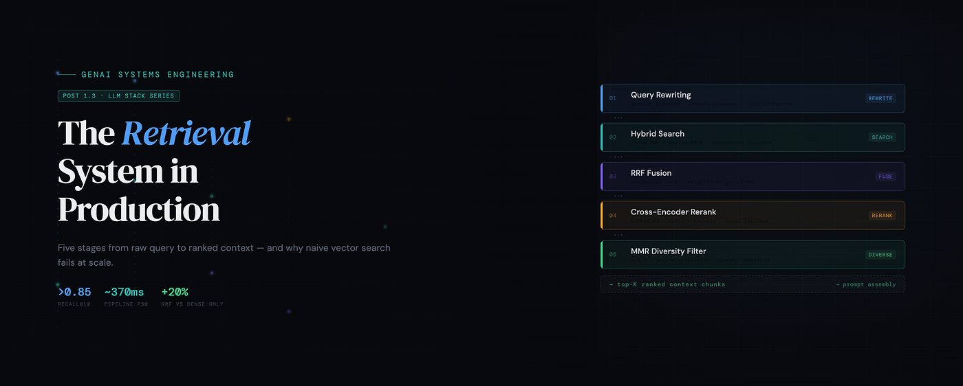
Retrieval is where most RAG systems silently fail. Not with errors — with quiet degradation. The vector search returns results, the prompt fills with context, the model produces an answer, and nobody notices that the retrieved chunks were loosely relevant at best and completely wrong at worst. The hallucination rate climbs. The grounding score drifts downward. The engineering team ships a new model version looking for gains and finds none, because the problem was never the model.

A production retrieval system is not a vector database wrapper. It’s a five-stage pipeline with compounding quality decisions: query rewriting before embedding, hybrid dense-plus-sparse search, metadata filtering as a hard constraint layer, cross-encoder re-ranking to promote precision, and result diversity enforcement to prevent context windows dominated by near-duplicate chunks. Each stage addresses a distinct failure mode. Skip any one of them and you’re leaving recall or precision on the table.

This post walks through all five, with the implementation details and the latency math that determines whether each stage earns its place in your pipeline.

Post 1.3 in the Anatomy of a Production LLM Stack series. Post 1.1 covered the API gateway layer. Post 1.2 covered orchestration — state machines, parallel DAG dispatch, and retry semantics. This post covers the retrieval system, which runs as a DAG branch within the orchestration layer’s RETRIEVING state.

The Five-Stage Retrieval Pipeline

Before diving into each stage, here is the complete picture. A query enters the retrieval system as raw user text and exits as an ordered, deduplicated, diversity-enforced list of the most relevant chunks for prompt assembly. Every stage adds latency and every stage is justified by the recall or precision gain it provides.

Fig 1. The five-stage production retrieval pipeline. Each stage adds latency but addresses a distinct failure mode that the previous stage cannot catch. The total p50 of ~370ms is dominated by query rewriting and re-ranking — both removable for latency-critical paths at a quality cost.

Stage 1 — Query Rewriting Before Embedding

The embedding model you use to encode queries was trained on clean, well-formed sentences. User queries are frequently none of those things. They’re short, ambiguous, domain-abbreviated, or context-dependent in ways that only make sense when you know what the user has been doing for the past three turns. “What was the revenue?” is five tokens that embed somewhere near the centroid of “revenue” — not anywhere near “Q3 2024 ARR breakdown by segment,” which is where the relevant document chunk lives.

Query rewriting is a lightweight LLM call — always to a small model like gpt-4o-mini or claude-haiku — that expands the raw query into a retrieval-optimized form before it reaches the embedding model. The rewriter is given the conversation history, any domain-specific terminology glossary, and a prompt that instructs it to produce a self-contained, specific query. The output is longer, more explicit, and embeds much closer to the target document space.

At 80ms and $0.0002 per query, the objection to query rewriting is always latency. The counter is that the re-ranked retrieval stage costs 160ms regardless. If better queries mean the re-ranker sees more relevant candidates in its top-20, the re-ranker promotes the right chunks to the top-5. Better context means fewer model retries, fewer hallucinations, and fewer escalations to the frontier model. The math overwhelmingly favors rewriting.

from dataclasses import dataclass
from typing import Optional

REWRITE_SYSTEM = """You are a retrieval query optimizer. Given a user query and recent conversation context, rewrite the query into a self-contained, retrieval-optimized form. The rewritten query should:
- Resolve all pronouns and implicit references
- Expand domain abbreviations using the glossary provided
- Include specific entity names, time ranges, or metric names if inferable
- Be 1–3 sentences maximum

Return ONLY the rewritten query. No explanation."""

@dataclass
class RewriteResult:
    original: str
    rewritten: str
    expanded: bool  # True if meaningful expansion occurred

async def rewrite_query(
    query: str,
    history: list[dict],
    glossary: dict[str, str],
    model: str = "claude-haiku-4-5-20251001",  # always use cheap model
) -> RewriteResult:
    context_block = "\n".join(
        f"{m['role'].upper()}: {m['content'][:200]}"  # truncate history
        for m in history[-4:]  # last 4 turns only
    )

    glossary_block = "\n".join(f"  {k}: {v}" for k, v in glossary.items())

    prompt = f"""Conversation context:
{context_block}

Domain glossary:
{glossary_block}

User query: {query}

Rewritten query:"""

    response = await llm_client.complete(
        model=model,
        system=REWRITE_SYSTEM,
        user=prompt,
        max_tokens=200,
        temperature=0.0,  # deterministic rewrites only
    )

    rewritten = response.content.strip()

    # Fall back to original if rewrite is suspiciously short or unchanged
    if len(rewritten) < len(query) * 0.8 or rewritten.lower() == query.lower():
        return RewriteResult(original=query, rewritten=query, expanded=False)

    return RewriteResult(original=query, rewritten=rewritten, expanded=True)

Set temperature=0.0 on your rewriter. A rewriter with any temperature will occasionally hallucinate entity names, dates, or metric names that don't exist in your corpus. Those hallucinated terms embed into regions of vector space with no matching documents, and your retrieval silently returns nothing relevant. Deterministic rewriting only.

Stage 2 — Hybrid Search: Dense Plus Sparse

Pure vector (dense) search is excellent at semantic similarity. Ask “what are the side effects of this medication” and ANN retrieval will find documents that discuss adverse reactions, contraindications, and warnings even if those exact words don’t appear. What it cannot do is reliably find a chunk containing the string ERR_CONNECTION_REFUSED, a SKU like XR-4421-BLK, or a person's name — entities that have precise string representations and need to be matched exactly.

Pure BM25 (sparse) search is the complement: exact term matching with TF-IDF weighting. It finds your ERR_CONNECTION_REFUSED with perfect recall. It completely fails on "what went wrong with the network connection" because there's no term overlap. Production retrieval systems run both in parallel and merge results using Reciprocal Rank Fusion (RRF).

Fig 2. Parallel dense + sparse retrieval merged via Reciprocal Rank Fusion. Both paths run concurrently; wall-clock time equals the slower path (dense ANN at ~120ms). RRF avoids needing to normalize scores across different retrieval systems.

RRF is elegant because it sidesteps the hardest problem in hybrid search: how do you combine a cosine similarity score (range 0–1, meaning-dependent) with a BM25 score (unbounded, corpus-dependent) into a single merged ranking? The answer is to ignore the scores entirely and use only the ranks. Each document’s RRF score is the sum of 1 / (k + rank) across all retrieval lists it appears in, where k=60 is a smoothing constant. A document ranked #1 in both lists scores much higher than one ranked #1 in only one list. Documents absent from a list contribute 0 for that list.

import asyncio
from dataclasses import dataclass, field
from typing import Any

ABSENT_RANK = 9999  # sentinel value for missing rank

@dataclass
class RetrievedChunk:
    chunk_id: str
    content: str
    metadata: dict
    dense_rank: int = ABSENT_RANK
    sparse_rank: int = ABSENT_RANK
    rrf_score: float = 0.0

def _compute_rrf_contribution(weight: float, rank: int, k: int) -> float:
    return weight * (1.0 / (k + rank))

def reciprocal_rank_fusion(
    dense_results: list[RetrievedChunk],
    sparse_results: list[RetrievedChunk],
    k: int = 60,
    dense_weight: float = 0.6,  # tunable per query type
    sparse_weight: float = 0.4,
) -> list[RetrievedChunk]:
    scores: dict[str, float] = {}
    index: dict[str, RetrievedChunk] = {}

    for rank, chunk in enumerate(dense_results, start=1):
        chunk.dense_rank = rank
        scores[chunk.chunk_id] = scores.get(chunk.chunk_id, 0.0) + _compute_rrf_contribution(dense_weight, rank, k)
        index[chunk.chunk_id] = chunk

    for rank, chunk in enumerate(sparse_results, start=1):
        chunk.sparse_rank = rank
        scores[chunk.chunk_id] = scores.get(chunk.chunk_id, 0.0) + _compute_rrf_contribution(sparse_weight, rank, k)
        index.setdefault(chunk.chunk_id, chunk)  # sparse-only chunks

    for chunk_id, score in scores.items():
        index[chunk_id].rrf_score = score

    return sorted(index.values(), key=lambda c: c.rrf_score, reverse=True)

async def hybrid_search(
    query_embedding: list[float],
    query_text: str,
    top_k: int = 20,
    dense_weight: float = 0.6,
) -> list[RetrievedChunk]:
    dense_results, sparse_results = await asyncio.gather(
        ann_search(query_embedding, top_k=top_k),
        bm25_search(query_text, top_k=top_k),
    )

    return reciprocal_rank_fusion(
        dense_results,
        sparse_results,
        dense_weight=dense_weight,
        sparse_weight=1.0 - dense_weight,
    )

The dense_weight and sparse_weight parameters are not set once and forgotten. In a production system, the query classifier (from the orchestration layer) should set these dynamically per query type. Exact-match queries (error codes, SKUs, names) should lean sparse (0.3/0.7 or even 0.0/1.0). Semantic queries (conceptual questions, summaries) should lean dense (0.7/0.3). Keeping this tunable per query type is what separates a production hybrid search from a naive one.

Stage 3 — Metadata Filtering as a Hard Constraint

Retrieval systems should never return results across tenant boundaries. This sounds obvious but is violated constantly in naive implementations where metadata filtering is applied as a post-processing step to the vector search results rather than as a pre-condition of the search itself.

The difference matters. If you retrieve the top-20 results from your entire corpus and then filter to the requesting tenant’s documents, you’ve potentially returned 0 results — because all 20 happened to belong to other tenants. Worse, you’ve wasted the query on irrelevant space. Production metadata filtering uses pre-filter constraints: the vector database query includes the metadata filter as part of the search predicate, restricting the candidate set before ANN distance computation begins.

from dataclasses import dataclass
from datetime import datetime
from typing import Optional

@dataclass
class MetadataFilter:
    tenant_id: str
    doc_types: Optional[list[str]] = None   # e.g. ['report', 'policy']
    date_after: Optional[datetime] = None   # freshness constraint
    date_before: Optional[datetime] = None
    access_level: Optional[str] = None      # 'public' | 'internal' | 'restricted'

    def to_qdrant_filter(self) -> dict:
        # Always start with tenant isolation
        must: list[dict] = [
            {"key": "tenant_id", "match": {"value": self.tenant_id}}
        ]

        if self.doc_types:
            must.append({"key": "doc_type", "match": {"any": self.doc_types}})

        if self.date_after:
            must.append({"key": "created_at", "range": {"gt": self.date_after.timestamp()}})

        if self.date_before:
            must.append({"key": "created_at", "range": {"lt": self.date_before.timestamp()}})

        if self.access_level:
            must.append({"key": "access_level", "match": {"value": self.access_level}})

        return {"must": must}

    def _build_date_range(self) -> Optional[dict]:
        if not (self.date_after or self.date_before):
            return None

        bounds: dict = {}
        if self.date_after:
            bounds["gt"] = self.date_after.isoformat()
        if self.date_before:
            bounds["lt"] = self.date_before.isoformat()

        return {"range": {"created_at": bounds}}

    def to_elasticsearch_query(self) -> dict:
        # Elasticsearch / OpenSearch BM25 filter format
        filters: list[dict] = [
            {"term": {"tenant_id": self.tenant_id}}
        ]

        if self.doc_types:
            filters.append({"terms": {"doc_type": self.doc_types}})

        if date_range := self._build_date_range():
            filters.append(date_range)

        return {"bool": {"filter": filters}}

Tenant isolation in metadata filtering is a security boundary, not a quality optimization. Any retrieval path that can return documents across tenant boundaries is a data isolation failure. The tenant_id filter must always be in the must clause — never in should. Audit this assumption in every code path, including fallback paths triggered by vector DB errors.

Stage 4 — Cross-Encoder Re-Ranking

The top-20 results from hybrid search have good recall — they likely contain the relevant chunks. But their order is determined by ANN distance and BM25 score, neither of which captures the full semantic relationship between the query and a specific chunk. A cross-encoder re-ranker takes each (query, chunk) pair and scores it jointly using a model that sees both simultaneously, rather than comparing separate embeddings.

This is the key architectural distinction. Bi-encoder retrieval (standard ANN) encodes query and document independently and measures similarity in the embedding space. Cross-encoder scoring encodes both together, allowing the model to reason about their relationship directly. Cross-encoders are slower — they cannot be pre-computed — which is why they’re applied only to the top-20 candidates, not the entire corpus. The compute cost is O(top_k), not O(corpus_size).

Fig 3. Each stage compounds the previous gain. Dense-only retrieval achieves 0.61 recall@10. The full five-stage pipeline reaches 0.88 — a 44% relative improvement. Benchmarked on a mixed corpus of enterprise documents with both semantic and keyword query types.

import asyncio
from typing import Optional

COHERE_OVER_FETCH_MULTIPLIER = 2  # over-fetch for diversity filter

async def rerank(
    query: str,
    candidates: list[RetrievedChunk],
    top_n: int = 5,
    model: str = "rerank-english-v3.0",
    score_threshold: float = 0.3,  # discard below-threshold results
) -> list[RetrievedChunk]:
    """Rerank candidates via Cohere Rerank API (cross-encoder)."""
    if not candidates:
        return []

    response = await cohere_client.rerank(
        query=query,
        documents=[c.content for c in candidates],
        top_n=min(top_n * COHERE_OVER_FETCH_MULTIPLIER, len(candidates)),
        model=model,
        return_documents=False,  # we already have the documents
    )

    return [
        _apply_rerank_score(candidates[result.index], result.relevance_score)
        for result in response.results
        if result.relevance_score >= score_threshold
    ]

async def local_rerank(
    query: str,
    candidates: list[RetrievedChunk],
    top_n: int = 5,
) -> list[RetrievedChunk]:
    """Fallback reranker using bge-reranker-large via HuggingFace endpoint."""
    pairs = [(query, c.content) for c in candidates]
    scores = await hf_endpoint.score_pairs(pairs, model="BAAI/bge-reranker-large")

    for chunk, score in zip(candidates, scores):
        chunk.rerank_score = score

    return sorted(candidates, key=lambda c: c.rerank_score, reverse=True)[:top_n]

def _apply_rerank_score(chunk: RetrievedChunk, score: float) -> RetrievedChunk:
    chunk.rerank_score = score
    return chunk

Stage 5 — Result Diversity Enforcement

After re-ranking, your top-5 results can easily be five versions of the same document chunk — the same paragraph from the same PDF, extracted at five slightly different chunk boundaries during indexing. The model sees this as a single piece of evidence repeated five times. It over-weights that evidence relative to other relevant documents that didn’t make the top-5 due to chunking accidents.

Maximal Marginal Relevance (MMR) is the standard approach. It selects results iteratively: pick the highest-scoring unselected result, then at each subsequent step pick the result that maximizes the combination of relevance to the query and dissimilarity to already-selected results. The trade-off between relevance and diversity is controlled by a parameter λ.

import numpy as np

_EPSILON = 1e-8  # numerical stability guard for cosine similarity

def cosine_similarity(a: list[float], b: list[float]) -> float:
    a_arr, b_arr = np.array(a), np.array(b)
    return float(np.dot(a_arr, b_arr) / (np.linalg.norm(a_arr) * np.linalg.norm(b_arr) + _EPSILON))

def _mmr_score(
    candidate: RetrievedChunk,
    selected: list[RetrievedChunk],
    lambda_param: float,
) -> float:
    """Compute MMR score: weighted combination of relevance and diversity."""
    relevance = candidate.rerank_score
    max_sim = max(cosine_similarity(candidate.embedding, s.embedding) for s in selected)
    return lambda_param * relevance - (1 - lambda_param) * max_sim

def maximal_marginal_relevance(
    candidates: list[RetrievedChunk],
    top_n: int = 5,
    lambda_param: float = 0.6,  # 1.0 = pure relevance, 0.0 = pure diversity
) -> list[RetrievedChunk]:
    """
    MMR selection — balances relevance with diversity.
    Requires each chunk to have a pre-computed embedding vector.
    """
    if not candidates:
        return []

    remaining = list(candidates)
    selected: list[RetrievedChunk] = [remaining.pop(0)]  # seed with highest-relevance result

    while len(selected) < top_n and remaining:
        best_chunk = max(remaining, key=lambda c: _mmr_score(c, selected, lambda_param))
        selected.append(best_chunk)
        remaining.remove(best_chunk)

    return selected

Set lambda_param=0.6 as your baseline. This weights relevance 60% and diversity 40%, which works well for most enterprise RAG use cases. For question-answering where a single precise answer is expected, raise it toward 0.8. For research-style queries where coverage across multiple sources matters, lower it toward 0.4. Add this as a per-query-type tunable parameter, not a system constant.

The Silent Killer: Embedding Model Drift

You’ve built the five-stage pipeline. It’s performing well. Then three months later, the embedding model provider releases a new version. You update your query encoder. Your retrieval quality silently collapses.

Embedding model drift is the most insidious failure mode in production retrieval systems because it produces no errors. The vector database returns results, RRF merges them, the re-ranker scores them. But the query embedding now lives in a slightly different vector space than the document embeddings indexed with the previous model version. Cosine similarity scores drop. The top-20 candidates are worse. Re-ranking can’t save you because the input pool is already degraded.

Always pin your embedding model version in production. text-embedding-3-large and text-embedding-3-large-v2 are not compatible. Documents indexed with one cannot be reliably searched with the other. Major embedding providers allow version pinning via model string — use it. When you do need to migrate, re-index incrementally: update a shadow index with the new model, validate recall@10 against your eval set, then swap. Never in-place migrate a production index.

Key Metrics at the Retrieval Layer

What Comes Next

Post 1.4 covers prompt assembly — the step that takes the top-K results from this retrieval pipeline and constructs the exact token sequence sent to the model. Prompt assembly is where context budget management, injection security, and template versioning live. Most teams treat it as string formatting. It isn’t.

If you found this post informative, please feel free to send me a connection request on LinkedIn.

If you found something missing, or wrong, please let me know in the comments so that everybody stays on the same page.