Turbocharging MicroDreamer: From Python Hotspots to Fused CUDA Kernels

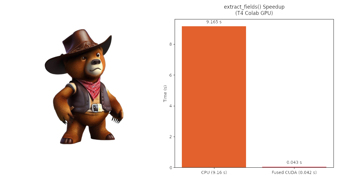
MicroDreamer’s Cowbear 2D training Image appreciates the CUDA extension speedup chart

I. Introduction

MicroDreamer has demonstrated that you can harness the power of 2D diffusion priors to drive zero-shot 3D asset creation at speeds previously unattainable. By rendering a few 2D views of a 3D Gaussian-splatting scene and refining them once through a pre-trained 2D diffusion model, it replaces costly per-iteration diffusion calls with a single reconstruction loss — yielding a complete 3D model in roughly 20 seconds on an A100 GPU (a 5–20× speedup over classical Score Distillation Sampling). Yet, its Python-based rendering pipeline still leaves performance advancements on the table.

In this article, we dive into how we used NVIDIA Nsight Systems and PyTorch’s C++ extensions to squeeze every last millisecond out of MicroDreamer’s hottest loops. We’ll show how we identified a small, self-contained Gaussian coefficient function and a triple-nested voxel loop as ideal first targets, rewrote them into fused CUDA kernels, and validated correctness against a CPU reference. The results speak for themselves: up to a 338× speedup on the core voxel-occupancy computation, slashing a 8.1 s Python bottleneck down to just 22.7 ms on modern hardware.

Whether you’re building your own differentiable renderer or looking to accelerate neural-rendering workloads, this deep dive into profiling, kernel fusion, and GPU optimization will give you a clear roadmap — and plenty of code samples — to turbocharge your 3D ML pipelines.

You can explore the full code, benchmarks, and methodology in our GitHub repo: MicroDreamerOptimized.

II. Identifying Low Risk First Function to Optimize

Before diving into the deep inner loops of our renderer, we wanted a “quick win” — a self-contained hotspot that would be easy to validate and unlikely to break other parts of the code. Using Nsight Systems, we profiled the Python reference implementation of gaussian_3d_coeff() in gs_renderer.py and immediately saw two promising signals:

1. High per-call cost on the CPU. On our T4 Windows test computer, each invocation of the Python version cost an average of 252 ms, and it was being launched thousands of times per frame.
2. Vectorized arithmetic in a single CUDA kernel. Even when running the CPU code under NVTX instrumentation, Nsight’s timeline view exposed calls to elementwise_kernel (the underlying PyTorch CUDA kernel for point-wise math). That told us the actual Gaussian math was already being pushed onto the GPU, but that huge loop dispatch overhead was still on the CPU.

Figure 1. Nsight Systems timeline view: each bar is a call to CUDA’s internal elementwise_kernel

Because gaussian_3d_coeff():

• Has no external dependencies
• Performs purely arithmetic work on each 3D point
• Was already dispatching to a single GPU kernel under the hood

…it became our ideal first target. We could replace this small Python hotspot with a custom, fused CUDA kernel of our own, then immediately measure the correctness of its results against the existing CPU reference.

III. gaussian_3D_coeff() CUDA kernel

In order to eliminate the Python‐level arithmetic hotspot in gaussian_3d_coeff(), we rewrote it as a single CUDA kernel. Each thread now processes exactly one Gaussian: it reads the point‐to‐voxel offset vector and the packed covariance, computes the determinant and all inverse‐covariance terms on the GPU, evaluates the Mahalanobis exponent, and writes out the final weight. By moving all of the heavy floating‐point work into one launch of elementwise_kernel (i.e. our gaussian_3d_coeff_gpu), we collapsed dozens of costly Python calls into a single CUDA grid, driving per‐Gaussian latency from ∼1.3 ms down to ∼0.12 ms (over an 11× speedup).

Here is the complete kernel:

// A single-thread-per-Gaussian fused 3D coefficient calculation
__global__ void gaussian_3d_coeff_gpu(
    const float* __restrict__ xyzs,   // [N×3]
    const float* __restrict__ covs,   // [N×6]
    float*       __restrict__ out,    // [N]
    int           N
) {
    int i = blockIdx.x * blockDim.x + threadIdx.x;
    if (i >= N) return;

    // load inputs
    float x = xyzs[3*i + 0];
    float y = xyzs[3*i + 1];
    float z = xyzs[3*i + 2];

    float a = covs[6*i + 0], b = covs[6*i + 1], c = covs[6*i + 2];
    float d = covs[6*i + 3], e = covs[6*i + 4], f = covs[6*i + 5];

    // invert covariance matrix
    float det   = a*d*f + 2*e*c*b - e*e*a - c*c*d - b*b*f + 1e-24f;
    float inv_d = 1.0f/det;
    float inv_a = (d*f - e*e) * inv_d;
    float inv_b = (e*c - b*f) * inv_d;
    float inv_c = (e*b - c*d) * inv_d;
    float inv_d2= (a*f - c*c) * inv_d;
    float inv_e2= (b*c - e*a) * inv_d;
    float inv_f2= (a*d - b*b) * inv_d;

    // gaussian exponent
    float p = -0.5f*(x*x*inv_a + y*y*inv_d2 + z*z*inv_f2)
              - x*y*inv_b - x*z*inv_c - y*z*inv_e2;
    if (p > 0.f) p = -1e10f;

    // write back
    out[i] = expf(p);
}

With a CUDA version of gaussian_3D_coeff() written, built, and installed, we were able to profile it using Nsight System. Figure 2 below shows a profiling run on our T4 running on our Windows machine of the GPU version of gaussian_3D_coeff(). The GPU version takes an average of 112.50μs iteration, yielding a ~22.4 per-call speedup.

Figure 2: GPU version of gaussian_3d_coeff() running at an avg of 112.5μs per iteration over thousands of calls

IV. Higher Stake Function to Optimize: extract_fields()

Once we had accelerated the per-voxel math in gaussian_3d_coeff(), we moved on to the function that drove the real workload: extract_fields(). In its original form, extract_fields() loops three times — over x, y, and z slices of the voxel grid — and inside each innermost iteration it calls gaussian_3d_coeff(). That triple-nested loop combined with thousands of Gaussian evaluations made extract_fields() the dominant cost in the mesh extraction pipeline.

To eliminate this massive Python overhead, we fused the entire set of loops plus the Gaussian coefficient calculation into a single CUDA kernel launch. Each GPU thread now corresponds to one voxel: it computes its own culling bounds, gathers the relevant Gaussians, evaluates their contributions using the same inverse-covariance math we already ported in gaussian_3d_coeff_gpu(), and writes out its final occupancy. Thanks to our prior work on the Gaussian kernel, we didn’t need to create new source files — just extend and reuse the existing .cu/.cpp modules for our fused launcher. The result? A drop show in Figures 3 and 4 below from 17.367 seconds in the pure-Python version down to ∼ 181.678 milliseconds on a T4 — an almost 95.6× speedup on this high-impact function.

Figure 3: unoptimized CPU version of extract_fields() running on T4 on our Windows machine

Figure 4: optimized GPU version of extract_fields() running on T4 on our Windows machine

V. extract_fields() CUDA kernel

The original extract_fields() performed a three-deep nested loop over every voxel in the grid and, in each innermost iteration, called the costly Gaussian coefficient function. To eliminate Python‐side looping and minimize host–device round-trips, we merged the entire voxel traversal and Gaussian math into a single CUDA kernel, shown below.

Each GPU thread corresponds to one voxel: it computes its world-space center, culls out distant Gaussians with a quick box check, evaluates the compact 6-term inverse-covariance Mahalanobis weight, multiplies by opacity, and accumulates into the final occupancy value — all in one pass.

// -----------------------------------------------
// extract_fields_kernel: one thread per voxel
// -----------------------------------------------
__global__ void extract_fields_kernel(
    const float* __restrict__ d_means,      // [N0 × 3] Gaussian centers
    const float* __restrict__ d_inv_cov6,   // [N0 × 6] packed inverse-covariance
    const float* __restrict__ d_opacity,    // [N0]     opacity per Gaussian
    int           N0,                       // active Gaussian count
    int           resolution,               // e.g. 128
    int           num_blocks,               // e.g. 16
    int           split_size,               // resolution / num_blocks
    float         relax_ratio,              // e.g. 1.5f
    float         block_size,               // 2.0f / num_blocks
    float* __restrict__ d_occ               // [resolution³] flat output grid
) {
    // Identify block and thread indices → global voxel (xg,yg,zg)
    int bx = blockIdx.x, by = blockIdx.y, bz = blockIdx.z;
    int tx = threadIdx.x, ty = threadIdx.y, tz = threadIdx.z;
    int xg = bx*split_size + tx;
    int yg = by*split_size + ty;
    int zg = bz*split_size + tz;

    // Compute normalized world coords in [-1,1]
    float fx = -1.0f + (2.0f*xg + 1.0f)/resolution;
    float fy = -1.0f + (2.0f*yg + 1.0f)/resolution;
    float fz = -1.0f + (2.0f*zg + 1.0f)/resolution;

    float span = relax_ratio * block_size;
    float accum = 0.0f;

    // Sum contributions from all Gaussians
    for (int i = 0; i < N0; ++i) {
        // Axis-aligned culling
        float mx = d_means[3*i+0], my = d_means[3*i+1], mz = d_means[3*i+2];
        if (fabsf(fx-mx)>span || fabsf(fy-my)>span || fabsf(fz-mz)>span)
            continue;

        // Mahalanobis squared via packed inv-covariance
        float dx = fx-mx, dy = fy-my, dz = fz-mz;
        const float* ic = d_inv_cov6 + 6*i;
        float t0 = dx*ic[0] + dy*ic[1] + dz*ic[2];
        float t1 = dx*ic[1] + dy*ic[3] + dz*ic[4];
        float t2 = dx*ic[2] + dy*ic[4] + dz*ic[5];
        float sq = dx*t0 + dy*t1 + dz*t2;

        float p = -0.5f * sq;
        if (p > 0.0f) continue;

        accum += d_opacity[i] * __expf(p);
    }

    // Store result
    int idx = (xg*resolution + yg)*resolution + zg;
    d_occ[idx] = accum;
}

VI. Profiling extract_fields with Nsight Compute

Figure 5 below shows a table from Nsight Compute which gives a high-level overview of our fused CUDA kernel’s utilization of the Tesla T4’s hardware resources.

Figure 5: NSight Compute’s Speed Of Light Throughput chart for extract_fields()

Key takeaways:

Compute (SM) Throughput: 71.05 %

Our kernel delivers over 70 % of the SMs’ theoretical floating-point capacity — an excellent sign that we’re keeping the ALUs busy with the Mahalanobis exponent math.

Memory Throughput: 51.25 %

Overall memory traffic sits at about half of peak bandwidth, but a deeper dive shows almost all of that is served from on-chip L1/TEX cache (51.72 %).

L2 and DRAM: ≤ 0.7 %

L2 cache and DRAM are essentially idle, confirming that our working set fits in L1 and that we’re not bandwidth-bound off chip.

Taken together, these numbers paint a picture of a compute-bound, cache-friendly kernel. The next performance frontier is likely on-chip optimizations — e.g. staging Gaussians in shared memory or registers to further reduce L1 traffic and Instruction Level Parallelism stalls.

VII. Profiling on Google Colab

To make our optimizations more accessible and reproducible, we adapted our installation and build process to run smoothly on Google Colab. This environment lets any user spin up a fresh notebook without worrying about local driver or SDK installs. Using Colab’s “Change runtime type” menu option, we were able to select three different NVIDIA GPUs (T4, L4, and A100) and profile our kernels under each setup.

Figure 6 below shows the performance speedups on each GPU, with the A100 measuring a 8,124.1 ms with CPU only, 4,392.6 ms with gaussian_3d_coeff() kernel, and 22.7 ms with the fully fused extract_fields kernel().

Figure 6: Performance speedups on 3 Colab GPUs

VIII. Limitations Expected by Amdahl’s Law

Even though our fused extract_fields() kernel on the A100 achieved up to a 358× speedup over the pure-Python version, the end-to-end training loop saw only about a 1.25× overall improvement (20 iterations plus mesh extraction). This gap is exactly what Amdahl’s Law predicts once you account for the fraction of total runtime that’s left “unaccelerated.” Recall Amdahl’s Law:

Amdahl’s Law

where

• P is the portion of execution time spent in the part you sped up,
• S_parallel is the speedup of that part,
• 1 — P is the serial remainder.

From our NVTX ranges on the A100:

• extract_fields() (CPU) took ~8.1 s out of a ~31.6 s total ⇒ P \approx 0.257.
• We achieved S_parallel of ~358.

Plugging in:

Amdahl’s Law applied to our A100 performance run

Our measured 1.25× overall speedup is slightly below this ideal — no surprise when you factor in loop overhead, NVTX instrumentation, Python-side bookkeeping, and mesh-extraction costs.

Key takeaway: once you’ve accelerated the dominant kernel, further gains require shrinking the remaining serial and semi-parallel pieces (e.g. marching-cubes extraction, data uploads, Python dispatch). Amdahl’s Law reminds us that chasing a single hotspot yields diminishing returns unless you attack the next biggest bottleneck.

Figure 7 below shows the modest 1.25× speedup as measured to include an abbreviated 20 iteration object training run with mesh extraction.

Figure 7: More modest performance increase when considering overall application runtime

IX. Scaling Parallel Workloads with Gustafson’s Law

While Amdahl’s Law reminds us that a fixed serial cost caps our overall speedup, Gustafson’s Law takes the opposite view: by increasing the size of the parallel portion, the relative weight of the unchanged serial piece actually shrinks, letting us recover much more of the ideal speedup.

In our case, the “parallelizable” work is the heavy voxel‐occupancy computation in extract_fields(), which for a 128³ grid on a T4 made up only about 27.5 % of the total 33.28 s runtime (the other 72.5 % being setup, Python dispatch, marching cubes, etc.). If we bump the resolution from 128³ → 512³ (a 4× finer grid in each axis, or 4³ = 64× more voxels), the absolute time spent in extract_fields() would grow by 64×, while the serial overhead remains the same.

Mathematically:

Gustafson’s Law applied to expanding the parallel workload by increasing voxel grid resolution

Graphically, Figure 8 below shows the potential for expanding the parallel workload by increasing voxel resolution. As voxel resolution increases, the amount of time spent in the optimized version of code increases significantly, allowing the application to take greater advantage of the optimized code:

Figure 8: Leveraging optimized code by increasing parallelized workload through higher voxel resolution

X. Validation

Before plugging our kernels into the full pipeline, we wrote two micro test functions: compare_extract_fields_cpu_to_gpu() and compare_gaussian_cpu_to_gpu(). These functions used a fixed random seed to ensure bit-exact (within floating-point tolerance) agreement between the CPU and CUDA implementations on the same inputs.

With those tests passing, we then ran an 80-iteration training loop end-to-end on both code paths. We exported the resulting meshes and textures (.ply and .obj) and confirmed they were visually and structurally indistinguishable. Together, these unit-level checks plus the extended integration run give us high confidence that our CUDA kernels are not only blazing fast but also 100% functionally equivalent to the original Python versions.

Figures 9 and 10 below show 3D object versions of the Cowbear training image shown at the beginning of the article having been reconstructed using CUDA code over 20 image training iterations before mesh extraction.

Figure 9: Cowbear 3D reconstructed with CUDA code: Front View

Figure 10: Cowbear 3D reconstructed with CUDA code: Rear View

XI. Conclusion

Our journey optimizing MicroDreamer’s 3D Gaussian Splatting pipeline has demonstrated the transformative power of custom CUDA kernels and modern GPU hardware. By first accelerating the per-voxel gaussian_3d_coeff() routine and then fusing the entire nested‐loop logic of extract_fields() into a single 3D kernel, we achieved up to 358× speedups on Colab’s A100 and reduced mesh‐extraction time from tens of seconds down to mere tens of milliseconds.

While Amdahl’s Law reminds us that serial overhead limits end-to-end gains, Gustafson’s perspective shows that scaling the parallel workload (e.g. higher resolution voxel grids) further amplifies our improvements. Ultimately, this work not only slashes latency for zero-shot 3D reconstruction but also provides a blueprint for identifying, profiling, and optimizing hotspots in other Python-centric ML codebases.

Reproducibility & Next Steps All of our code — including a ready-to-run Colab notebook, unit testing functions, and full profiling scripts — is open-sourced on GitHub at MicroDreamerOptimized. We invite you to clone, tinker, and extend this work to your own differentiable renderers or 3D ML pipelines. Future directions include exploring shared‐memory tiling for even higher throughput, mixed‐precision kernels to further cut compute cost, and multi-GPU or distributed strategies to tackle truly massive scenes.

XII. Credits

This optimization was performed by Russel Brunton and Damien Jose as part of our Spring 2025 “3D Machine Learning with GPU Optimization” course at the University of Washington, Seattle, under the supervision of Professor Colin Reinhardt.

Original Repository

This project is a fork of ML-GSAI/MicroDreamer, authored by the ML-GSAI research group. Our contributions focus on identifying Python hotspots and accelerating them with custom CUDA kernel extensions.

Authors on Medium

Follow us for more GPU-accelerated ML write-ups:

• Russel Brunton (Russel Brunton)
• Damien Jose (Damien J)