Distribution Fitting Is Not the Problem: Structural Assumptions Dominate Model Risk

Article 6 of 8 — Can We Price GDPR Risk?

Summary. This article builds a reproducible procedure for estimating GDPR expected loss from public enforcement data. Base calibration (2018–2026, λ = 0.16%) yields an annual pure risk premium of €7,516 and a conditional mean severity of €4.4 million (P95 ≈ €8.8 million) for a non-platform commercial insured. The single largest modelling choice is not the severity distribution — it is the calibration window: restricting to the post-2023 enforcement regime increases the base premium by a factor of 3.7. The most important result is not the €7,516 figure. It is that the uncertainty surrounding GDPR pricing is itself measurable. The procedure does not eliminate uncertainty; it makes it observable.

The previous five articles built the empirical foundation. Article 2 documented the severity structure of GDPR enforcement: a Gini coefficient of 0.99, a mean-to-median ratio of 269:1, and a distribution in which the top 1% of cases account for 88% of all fine volume. Article 3 showed that enforcement frequency is overdispersed, jurisdiction-dependent, and separated from breach occurrence by a conversion funnel with a rate below 0.5%. Article 4 established that the academic literature on cyber insurance modelling has not produced an empirically calibrated framework for GDPR regulatory liability. Article 5 documented the structural concentration of GDPR exposure: three corporate groups account for 71% of all recorded fines; one supervisory authority — the Irish DPC — accounts for 66.6% of total fine volume.

The evidence is sufficient. The question is no longer whether GDPR enforcement is modelable. It is whether a model can be built from available public data in a way that is transparent enough to be useful and honest enough to be taken seriously.

This article proposes an auditable procedure for estimating GDPR expected loss using publicly available enforcement data. It does not estimate the true expected loss of any European company. It claims something narrower and more defensible: that the publicly available data supports a structured, reproducible estimation procedure — one that is conditional on stated assumptions, reproducible by any analyst with access to the same data, and updatable as new enforcement decisions accumulate.

Section 1 — Why a Procedure, Not a Prediction

The distinction between a procedure and a prediction matters here more than it usually does.

A prediction claims to describe what will happen. It can be falsified by a single counterexample. A pricing procedure claims to describe a method for converting available data into a defensible expected loss estimate — one that is conditional on stated assumptions, reproducible by any analyst with access to the same data, and updatable as the enforcement record grows.

Every existing GDPR fine carries explicit information: the jurisdiction, the fine amount, the date, the violation type, and the name of the sanctioned entity. This is more structured public data than exists for most long-tail liability categories at comparable stages of market development. The procedure built below uses nothing else.

What it cannot use — because it does not exist publicly — is an audited count of GDPR-exposed firms, a matched dataset linking breach notifications to enforcement outcomes at the entity level, or proprietary claims data from insurers who have written GDPR coverage. These absences are not incidental. They are the reason no pricing framework currently exists. Acknowledging them upfront is not a weakness of this procedure. It is a condition of its intellectual honesty.

Section 2 — What This Model Cannot Do

Before presenting the model, a clear account of its limitations is necessary. This is not a conventional disclaimer. In insurance modelling, the list of what a model cannot do is at least as important as what it can do — it defines where the model breaks and what happens to a practitioner who uses it outside its range.

An auditable model is not necessarily a correct model. It is a model whose data sources, assumptions, and calibration choices are explicit enough that another analyst can reproduce, critique, and modify the result. Auditability is therefore a property of the procedure, not of the output. The value of auditability is not accuracy — it is the ability to trace any result back to a specific assumption and to replace that assumption with a better one when better data becomes available.

This model cannot estimate four things:

True population frequency. The model is calibrated from observed enforcement outcomes, not from a known population of GDPR-exposed firms. No public dataset exists that identifies all EU data controllers with sufficient precision to serve as a frequency denominator. The frequency layer should therefore be interpreted as an empirical enforcement rate conditional on the available data — not as a true population frequency. The sensitivity of every downstream result to this limitation is shown explicitly in Section 6.

Civil liability under Article 82. GDPR Article 82 creates a parallel right to compensation for data subjects who suffer material or non-material damage. The CJEU has progressively expanded the scope of this right — Österreichische Post (2023), Scalable Capital (2024), and the German mass litigation following the 2024 Facebook-scraping ruling have opened a channel for aggregate claims that may ultimately dwarf the regulatory fine itself. This model covers regulatory fines only. The civil liability layer is addressed in Article 7.

Accumulation across policyholders. As Article 5 documented, GDPR enforcement is structurally concentrated at the entity and jurisdiction level. The model below treats each calibration anchor as an independent exposure. A reinsurer applying per-entity figures without an accumulation adjustment will systematically underestimate correlated exposure.

Development lag. GDPR investigations are long. The noyb case data shows approximately 30% of complaints remain unresolved after four years. The model uses enforcement dates, not incident dates. The IBNR problem this creates is addressed in Article 7.

Section 3 — Model Architecture

The model has three layers. They must be kept separate: collapsing any two produces a model that breaks when the underlying mix of jurisdictions, entity types, or enforcement pathways changes.

Layer 1: Frequency. How often does an enforcement event — a decision resulting in a fine — occur per controller per year?

The CMS enforcement tracker records approximately 406 fine decisions per year over the 2023–2024 period. Converting this to a per-controller rate requires a denominator — the size of the at-risk population — for which no definitive public figure exists. Three assumptions are presented. None is claimed to be correct. The reader should select or replace them based on their own portfolio context.

The relationship between frequency assumption and expected loss is linear: halving the denominator doubles the premium. This can be expressed directly as:

premium_adjusted = €7,516 × (250,000 / N_at_risk)

where N_at_risk is the at-risk population assumption relevant to the reader’s portfolio. Underwriters with proprietary enforcement experience in their book should replace 250,000 with their own estimate. Those without it should stress-test across the full 0.04%–0.41% λ range before anchoring any pricing decision.

Layer 2: Conversion. As Article 3 established, the breach-to-fine conversion rate is approximately 0.25% at the system level. For this model, conversion is embedded in the frequency layer: the λ figures above are calibrated to observed enforcement outcomes, not to breach notification counts.

Layer 3: Severity. Given that enforcement occurs, what is the distribution of the resulting fine?

Three distributional specifications are tested against the calibration anchor sample described in Section 4:

• Lognormal: Full maximum-likelihood fit. Parameters: μ = 10.58, σ = 3.04. AIC = 23,868.
• Spliced (Base): Lognormal body up to the 95th percentile (€4.42M threshold); Generalised Pareto Distribution above. Parameters: body μ = 10.29, σ = 2.84; tail ξ = 0.46, β = €4.32M. AIC = 23,583.
• Pareto-heavy: Lower threshold at the 75th percentile (€387k); heavier Pareto tail. Parameters: ξ = 0.926, β = €886k.

The AIC favours the spliced specification. With N = 910, distributional ambiguity is expected; the three specifications make that ambiguity explicit rather than suppressing it.

Expected loss structure:

The model produces two outputs that must be read together:

• Pure risk premium: the unconditional expected annual loss per controller — the actuarially correct premium base before loadings. At λ = 0.16%, the median annual loss is zero. The mean is not.
• Conditional severity: the expected loss given that enforcement occurs — the relevant metric for limit and retention design.

Section 4 — Calibration Anchor

The model is calibrated against a reference case — a calibration anchor constructed from the central portion of the observed enforcement distribution.

Article 5 demonstrated that GDPR fine severity is dominated by a small number of large technology platforms. The objective of this model is different: it estimates expected loss for a non-platform commercial insured — a company that processes personal data in the ordinary course of business but is not a global advertising-funded platform, a social network, or a large-scale data broker.

The calibration anchor is therefore defined as all enforcement outcomes associated with controllers whose cumulative recorded fines fall between €100,000 and €50 million. The lower bound excludes the mass of small-fine cases that reflect a domestic SME enforcement pattern with limited insurance relevance. The upper bound excludes the platform outliers.

The resulting sample contains 388 controllers and 910 individual fine observations. Its composition by jurisdiction:

Spain accounts for 43% of case count but only 15% of fine volume, with a median of €30,000. The severity parameters of the calibration anchor are driven primarily by Italy, France, and the Netherlands, where median fines range from €300,000 to €2.1 million. Spain shapes the body count; it does not shape the severity distribution.

The calibration anchor is reproducible. Any analyst applying the same bounds to the same dataset will obtain the same sample. The bounds are assumptions; changing them is a legitimate challenge to the calibration, not to the procedure.

Section 5 — Expected Loss Results

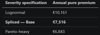
Applying the three severity specifications to the calibration anchor, with the illustrative midpoint frequency (λ = 0.16%), produces the following.

A) Pure Risk Premium (annual expected loss per controller — for pricing)

B) Conditional Severity (given enforcement occurs — for limit/retention design)

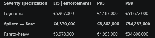
On the Lognormal row: why E[S] > P95. The conditional sample of enforcement events is sufficiently small that sampling variability remains material. With σ = 3.04, the lognormal distribution places non-trivial mass on extreme values. In any finite Monte Carlo sample drawn from this distribution, a small number of observations above €50 million can pull the empirical mean above the empirical 95th percentile of the same sample. The theoretical mean of LN(10.58, 3.04) is approximately €4.0 million; the theoretical P95 is approximately €5.8 million — the correct ordering. The inversion is a sampling artefact of a heavy-tailed distribution under finite simulation, not a model error. The P95 is the more stable estimator for limit design.

On the ordering of annual premiums. The Pareto-heavy specification produces a lower annual premium than the Lognormal — which may appear counterintuitive. The explanation lies in how the model is structured. The Pareto-heavy specification is not a nested version of the base model with a thicker tail added on top. It is a complete re-estimation of both body and tail structure under a different threshold assumption: lowering the threshold from the 95th to the 75th percentile assigns 25% of mass to the Pareto tail, but simultaneously re-fits the body component over a narrower, lower-severity range. A heavier tail does not mechanically imply a higher mean when the body is recalibrated at the same time. In a regime where enforcement occurs in fewer than 0.2% of controller-years, the annual premium is dominated by the body — not the tail. The tail matters for the P99, not for the mean. An underwriter reading only the annual premium column will draw the wrong conclusion: the Pareto-heavy specification is not a “low risk” scenario. It is a scenario in which rare events are more extreme but the annual average, driven by the recalibrated body, happens to be lower.

The base P95 conditional severity of €8.8 million is the number that matters for limit design. A mid-market GDPR policy with a €5 million limit does not cover the P95 outcome when enforcement occurs. A €10 million limit is marginally sufficient at P95 but leaves the P99 — €54 million under the base specification — unaddressed.

The ratio of conditional mean severity to annual pure premium is approximately 580:1. In professional liability, the equivalent ratio typically runs 20–50:1. This gap is the structural reason why standard liability pricing intuitions do not transfer to GDPR enforcement risk.

Section 6 — Distribution Fitting Is Not the Problem: Structural Assumptions Dominate Model Risk

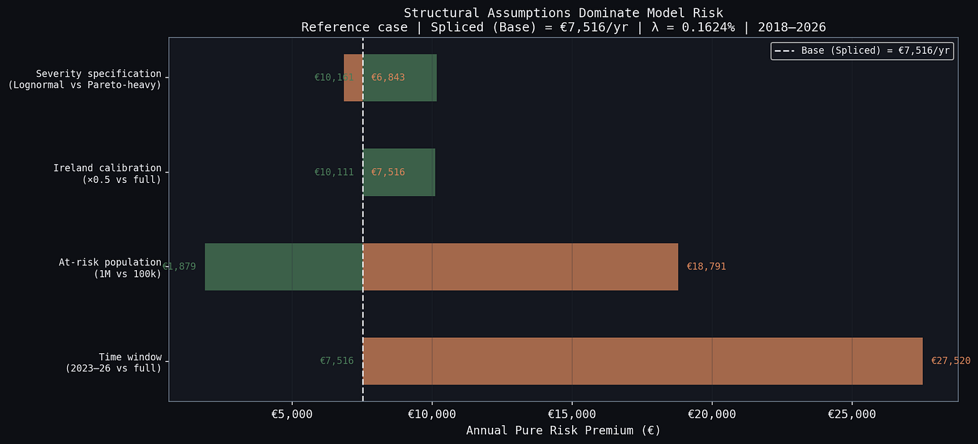
The four sensitivity levers are presented in order of impact. The ordering is not arbitrary — it reflects where the uncertainty in this model actually lives.

Time window: 3.7×

The base calibration uses the full 2018–2026 enforcement record. The year-by-year data reveals why this choice is consequential:

The average fine in 2023–2024 is approximately €4.0 million — roughly 2.5 times the 2021–2022 average and eight times the 2019–2020 average. Restricting the sample to 2023–2026 produces a pure premium of approximately €27,500: 3.7 times the base estimate of €7,516.

This is the single most consequential modelling choice in the procedure. The 2018–2020 period reflects GDPR’s ramp-up: supervisory authorities were building capacity, the One-Stop-Shop mechanism was not yet operational, and enforcement intensity was structurally lower. Including those years dilutes the severity calibration. Excluding them assumes the post-2023 regime is the forward-looking one.

Neither choice is obviously correct. But the 3.7× factor reveals something more important than any distributional assumption: the uncertainty in this model is not primarily statistical — it is structural. Which enforcement regime is the relevant one is a question no distribution fitting can answer.

Frequency assumption (λ): up to 10× across the full range

The λ assumption is the model’s most exposed parameter. No public data can close this uncertainty. The appropriate response is not to anchor on a single number but to stress-test across the full range and disclose the assumption explicitly when using any output for pricing decisions.

Ireland calibration: 1.35× (in an unexpected direction)

Downweighting Irish fines by 50% increases the pure premium from €7,516 to €10,111. The direction is counterintuitive. Removing large Irish fines from the top of the distribution shifts some controllers that were previously above the €50 million upper bound downward into the calibration anchor population, raising the body mean. This is a structural consequence of how concentration in the top tail creates pressure at the boundary of any bounded sample — not a modelling artefact.

Severity specification: ±35% around base

Moving from the spliced base to the lognormal-only specification increases the pure premium by approximately 35%. Moving to the Pareto-heavy specification decreases it by approximately 9%. The AIC strongly favours the spliced specification, but the practical impact of this choice is smaller than any of the three levers above.

Section 7 — Failure Modes

Four conditions would cause this model to break materially.

Failure Mode 1: Regulatory regime shift. The model is calibrated on historical enforcement data. A major EDPB coordinated decision — one establishing new precedent under Article 83(5) for systemic violations — could move the severity distribution discontinuously. The 3.7× time window sensitivity is a partial indicator of how quickly the regime can shift. Practical response: include a regulatory change clause; stress-test at 3.7× annually; trigger recalibration following any precedent-setting enforcement decision that materially exceeds the historical calibration range.

Failure Mode 2: Tail mis-specification. The base tail index ξ = 0.46 implies a finite-variance distribution. The Pareto-heavy specification’s ξ = 0.926 is approaching the region where variance becomes unstable — not infinite at this value, but increasingly sensitive to extreme observations. Expected loss estimates remain mathematically finite under all three specifications presented here, although they become progressively less stable as ξ approaches 1. This matters primarily for capital modelling and reinsurance layer pricing, not for primary limit adequacy. Practical response: for reinsurance structuring and capital allocation, stress-test alternative tail specifications including values near the upper confidence bound of the fitted ξ estimate; do not rely on mean estimates above the 95th percentile.

Failure Mode 3: Portfolio concentration. This model treats each calibration anchor as an independent exposure. As Article 5 documented, this assumption is violated in any real portfolio that includes controllers supervised by the Irish DPC, entities within the same corporate group, or companies with shared data infrastructure. A reinsurer applying per-entity figures without a DPA-level aggregation stress will systematically underestimate correlated exposure. Practical response: apply an Irish DPC stress scenario — assume three major decisions in a single calendar year — to any portfolio with material Irish-supervised exposure.

Failure Mode 4: Investigation lag. The model uses enforcement dates, not incident dates. Fines issued today may reflect breaches or complaints from three or four years ago. The IBNR reserve implied by the current pipeline of open investigations is not captured in any parameter in this model. Article 7 addresses this. Practical response: reserve for open investigations using a development pattern approach; do not treat zero reported losses in a given year as evidence of zero incurred losses.

What This Procedure Produces — and What It Does Not

The base calibration yields an annual pure risk premium of €7,516 for the reference case, conditional on the illustrative midpoint frequency assumption. The conditional severity, given enforcement, is €4.4 million at the mean and €8.8 million at the P95. The post-2023 calibration yields €27,500. The lower denominator assumption yields €18,790.

These are not competing answers to the same question. They are the correct outputs of a procedure applied under different, explicitly stated conditions. An analyst who disagrees with any assumption can replace it — the model accommodates that substitution directly, and the result changes in a quantifiable direction.

The most important result of this article is not the €7,516 figure. It is that the uncertainty surrounding GDPR pricing is itself measurable. The procedure does not eliminate uncertainty; it makes it observable. Every gap between the low and high estimates — the 3.7× from the calibration window, the 10× from the frequency denominator — is a gap that better data, proprietary claims experience, or improved regulatory transparency can close. Quantifying where the uncertainty lives is the first step toward closing it.

That is what an auditable pricing procedure is for.

Bridge to Article 7

The model built in this article is intentionally incomplete. Two loss layers are absent by design: the civil liability channel created by GDPR Article 82, and the development lag that separates enforcement dates from incident dates.

The civil liability omission is not minor. Preliminary analysis of the CJEU Article 82 jurisprudence suggests that, in a major data breach affecting a large number of data subjects, aggregate civil liability may substantially exceed the regulatory fine. A single enforcement event producing a €10 million fine may simultaneously trigger Article 82 claims across hundreds of thousands of affected individuals — a loss that this model, by construction, does not see.

Article 7 will quantify what this model is missing.

Data: CMS Law GDPR Enforcement Tracker (snapshot to April 2026), DLA Piper GDPR Fines Survey 2026. Code available in the Article 6 supplementary notebook.

Code: Colab notebook — reproduce all results from the Article 6 supplementary notebook.

About the Author

SukHee Lee is an analytics engineer specializing in insurance and data engineering, with experience in the (re)insurance sector. Holds a Master’s degree in Actuarial Science from Université Paris Diderot (ISIFAR). This series is an independent research project based entirely on publicly available data.

GitHub: github.com/SHLee5864