Mastering Array Partitioning and QuickSelect: A Guide to Efficient Algorithms
Unlock the secrets of efficient data manipulation with partitioning techniques and QuickSelect algorithms.
Mastering Array Partitioning and QuickSelect: A Guide to Efficient Algorithms
Unlock the secrets of efficient data manipulation with partitioning techniques and QuickSelect algorithms.
In the vast world of computer science, array manipulation stands as a foundational skill. Whether you’re sorting data, searching for specific elements, or optimizing performance, understanding how to partition arrays efficiently is crucial. In this guide, I’ll delve into the art of partitioning arrays and explore how the QuickSelect algorithm leverages these techniques to solve complex problems with remarkable efficiency.
Table of Contents
1. Introduction to Array Partitioning
1. Introduction to Array Partitioning
Partitioning an array involves rearranging its elements based on a specific condition or pivot, dividing it into distinct sections. This concept is the backbone of several efficient algorithms, including QuickSort and QuickSelect.
Imagine you have a deck of cards, and you want to separate them into red and black suits. Partitioning allows you to do this efficiently without needing to sort the entire deck.
2. Two-Way Partitioning
Understanding the Concept
Two-way partitioning divides an array into two sections based on a condition. For example:
• Even-Odd Partitioning: Place all even numbers before odd numbers or vice-versa.
• Pivot Partitioning: Place all elements smaller than or equal to a pivot before larger ones.
• Zero-First Partitioning: Move all zeros to the beginning of the array.
The Template
We’ll use a generic template inspired by the **Nico Lomuto partitioning scheme described in **Programming Pearls book: In such problems the array needs to be divided by a boundary separating the first partition and second partition. Let the index of this boundary be b1 all the indexes before this boundary belong to partition 1 and all the indexes after this boundary are either from partition 2 or unclassified. When a new element is seen while iterating the array, if the element belongs to first partition, the element is swapped by the b1, and then boundary is moved one step ahead. In such a way b1 identifies the first element of second partition.
def two_way_partition(A):
    b1 = 0  # Boundary index for partition one
    for i in range(len(A)):
      # The condition function determines whether an element belongs to the first partition.
        if condition(A[i]):
            # Element at i is part of parition 1, swap element at i and boundary index of partition 1
            swap(A, b1, i)
            # Now element at b1 is in partition 1 so increment b1
            b1 += 1
     # At the end of the loop
     # A[:b1] belong to partition 1
     # A[b1:] belong to partition 2
Practical Examples
Even-Odd Partitioning
def even_odd_partition(A):
    even_idx = 0
    for i in range(len(A)):
         # Condition: If the number is even
        if A[i] % 2 == 0:
            swap(A, even_idx, i)
            even_idx += 1
    # A[:even_idx] are even
    # A[even_idx:] are odd
Pivot Partitioning
def pivot_partition(A, pivot):
    idx = 0
    for i in range(len(A)):
        if A[i] <= pivot:
            swap(A, idx, i)
            idx += 1
    # A[:idx] <= pivot
    # A[idx:] > pivot
Zero-First Partitioning
def zero_first_partition(A):
    zero_idx = 0
    for i in range(len(A)):
        if A[i] == 0:
            swap(A, zero_idx, i)
            zero_idx += 1
    # A[:zero_idx] are all zero
    # A[zero_idx:] are != zero
Swap Function
def swap(A, i, j):
    A[i], A[j] = A[j], A[i]
3. Three-Way Partitioning
Extending the Concept
Three-way partitioning divides the array into three sections:
-
Elements belonging to partition one.
-
Elements belonging to partition two.
-
Unclassified or elements belonging to partition three.
The Template
def three_way_partition(A):
    b1 = b2 = 0
    for i in range(len(A)):
        # Is A[i] Belong to partition 1
        if condition1(A[i]):
            # Move A[i] to parition 1, by swaping it back.
            swap(A, b2, i)
            swap(A, b1, b2)
            b1 += 1
            b2 += 1
        # Is A[i] Belong to partion 2
        elif condition2(A[i]):
            swap(A, b2, i)
            b2 += 1
    # A[:b1] => Belong to partition 1
    # A[b1:b2] => Belong to partition 2
    # A[b2:] => Belong to partition 3
**Dutch National Flag Problem**
One of the most famous examples is the Dutch National Flag Problem, where we sort an array of 0s, 1s, and 2s.
def sortColors(nums: List[int]) -> None:
        """
        Do not return anything, modify nums in-place instead.
        """
        def swap(A: List[List[int]], i, j: int) -> int:
            A[i], A[j] = A[j], A[i]

        b1, b2, n = 0, 0, len(A)
        for i in range(n):
            if nums[i] == 0:
                swap(nums, b2, i)
                swap(nums, b1, b2)
                b2 += 1
                b1 += 1
            elif nums[i] == 1:
                swap(nums, b2, i)
                b2 += 1
    # nums[:b1] => Belong to partition 1 => 0
    # nums[b1:b2] => Belong to partition 2 => 1
    # nums[b2:] => Belong to partition 3 => 2
Now the same template can be applied to more partition problems like 4 way partition, only it would be more tedius to write.
4. QuickSelect
Quick select is the algorithm to select kth element in the array. It is uses the same techniques as in the Quick Sort where partitioning is done based on randomly selected index. With the difference that once the partition is decided based on the random selected pivot condition partition, only single recursive call with the desired partition is made. This makes the code to be tail recursive and thus can also be written iteratively.
Complexity of procedures like selecting the kth largest element or median in the list can be reduced to O(N) in the average case, with randomly chosen pivot, from the O(nlogn) naive solution of actually sorting the underlying structure.
How QuickSelect Works
QuickSelect is similar to QuickSort but focuses on calling partition function like discussed above, that could contain the desired element. The core of the problem is still the partition function with modifications, which is discussed earlier. So let’s look at the modifications.
def pivot_partition(A, lo, hi):
    # Get pivot index
    pi = random.randint(lo, hi)
    swap(A, pi, hi)
    b = lo
    for i in range(lo, hi):
        # Moves all the numbers smaller than selected pi to the left.
        if A[i] < A[hi]:
            swap(A, b, i)
            b+= 1
    swap(A, hi, b)
    return b
    # A[:b] > A[b]
    # A[b+1:] <= A[b]
In the partition function for quick select, a random pivot is selected and it’s position is determined by moving all the elements greater to the left of the pivot and all the elements smaller or equal to the right of the pivot. At the end the index of the pivot is returned.
Implementing QuickSelect
Quick select, gets or selects k th element in the sorted increasing order. This runs in O(n) average time, and uses the partition function described above. Usually the select body doesn’t change, the changes is mostly in the partition criteria which changes for different problems.
def quickSelect(nums: List[int], k: int) -> int:
    n = len(nums)
    lo, hi = 0, n - 1
    # k is 1-indexed
    k = k - 1
    while lo <= hi:
        pi = pivot_partition(nums, lo, hi)
        if pi < k:
            lo = pi + 1
        else:
            hi = pi - 1
    # when the loop stops, lo will be at the kth smallest element
    return nums[lo]
5. Real-World Applications
Let’s look at some leet code problems for different partition criteria.
**Finding the kth Largest Element**
Finding the kth largest element, is basically using quick select but finding the element from the end of the array. This can be done 1st largest element will be nothing but nth largest element in the sorted array, which can be given as n — k + 1
def findKthLargest(nums: List[int], k: int) -> int:
    return quickSelect(nums, len(nums) - k + 1)
In the leetcode the above times out in python for one of the use case, where there are lot of same elements in the input. The code can further optimized by partitioning it in three ways, such that smaller are on left and equal are in middle and greater are on right. Optimization here is if k is in the equal section then don’t need to run partition function again.
The next two problem solutions, have similar concepts with minor changes to the partition function. I have written in go, just to capture the concept in another language.
**K Closest Points to Origin**
Uses the same quick select as above by partitioning the points based on the manhattan distance from the origin. Once the kth element is found, returns the first kth element from the list.
func distance(point []int) int {
 return point[0]*point[0] + point[1]*point[1]
}

func partition(points [][]int, lo, hi int) int {
 pi := rand.Intn(hi-lo+1) + lo
 points[pi], points[hi] = points[hi], points[pi]
 pivot := distance(points[hi])
 for i := lo; i < hi; i++ {
  if distance(points[i]) < pivot {
   points[i], points[lo] = points[lo], points[i]
   lo++
  }
 }
 points[lo], points[hi] = points[hi], points[lo]
 return lo
}

func kClosest(points [][]int, k int) [][]int {
 // select body
 lo, hi := 0, len(points)-1
 for lo <= hi {
  p := partition(points, lo, hi)
  if p < k {
   lo = p + 1
  } else {
   hi = p - 1
  }
 }
 return points[:k]
}The partition function is modified here to work with the frequency of the item stored in the 1st index of the items list. Otherwise the select body is same.
func partition(items [][]int, lo, hi int) int {
    pi := rand.Intn(hi - lo + 1) + lo
    items[pi], items[hi] = items[hi], items[pi]
    b := lo
    for i := lo; i < hi; i++ {
        // highest and equal frequency items to the left of b
        if items[i][1] >= items[hi][1] {
            items[b], items[i] = items[i], items[b]
            b++
        }
    }
    items[b], items[hi] = items[hi], items[b]
    return b
}

func topKFrequent(nums []int, k int) []int {
    mp := map[int]int{}
    for _, v := range nums {
        mp[v]++
    }
    items := [][]int{}
    for v, f := range mp {
        items = append(items, []int{v, f})
    }
    // select body
    lo, hi := 0, len(items) - 1
    k = k - 1
    for lo <= hi {
        pi := partition(items, lo, hi)
        if pi < k {
            lo = pi + 1
        } else {
            hi = pi - 1
        }
    }
    // gathering results from items[:lo+1]
    sol := []int{}
    for i:= 0; i <= lo; i++ {
        sol = append(sol, items[i][0])
    }
    return sol
}
6. Conclusion
Mastering array partitioning and the QuickSelect algorithm opens doors to solving a myriad of problems efficiently. These techniques reduce time complexity and enhance performance, making them invaluable tools in any programmer’s arsenal.
Whether you’re preparing for coding interviews, optimizing applications, or just looking to deepen your understanding of algorithms, practicing these partitioning methods will undoubtedly pay off.
You can read more of my interview patterns here: https://adityabhatia.com/algos-ds/
Did you find this guide helpful? Share your thoughts and continue the conversation in the comments below!
메타데이터
- post_id
- 85a24dc89f36
- slug
- mastering-array-partitioning-and-quickselect-a-guide-to-efficient-algorithms-85a24dc89f36
- url
- https://medium.com/@tuubow/mastering-array-partitioning-and-quickselect-a-guide-to-efficient-algorithms-85a24dc89f36
- canonical_url
- https://medium.com/@tuubow/mastering-array-partitioning-and-quickselect-a-guide-to-efficient-algorithms-85a24dc89f36
- author_url
- https://medium.com/@tuubow
- status
- ok
- fetched_at
- 2026-06-12 07:40:50