Genes Before Gods: Reconstructing Ancient India Through Genetics Part 5

When India Stopped Mixing: How Chromosomes Recorded One of the Greatest Social Transformations in Indian History

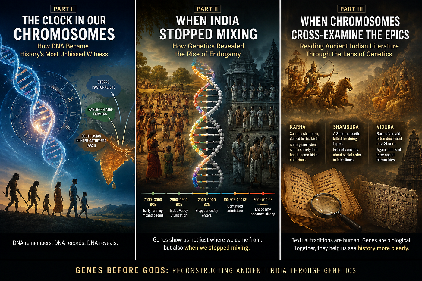
“History remembers kings. Chromosomes remember marriages.”

The Day the Chromosomes Fell Silent

Imagine that you are a chromosome. For thousands of years, your journey has been wonderfully chaotic.

You pass from one generation to the next, constantly exchanging pieces with other chromosomes through recombination. Your ancestors belonged to ancient hunter-gatherers who had lived in South Asia for tens of thousands of years. Later, other ancestors arrived carrying ancestry related to early farming communities from the Iranian plateau. Centuries passed. New people entered from the Eurasian Steppe. Every generation brought new encounters, new marriages and new mixtures.

You became a mosaic. Tiny pieces of many different ancestral histories became stitched together into a single chromosome. Generation after generation, recombination continued quietly, almost mechanically, with no concern for language, religion, occupation or social status.

Then, something unexpected happened.

The steady reshuffling began to slow. Not because recombination stopped. Biology never stopped doing its work. It slowed because people stopped choosing partners from outside their own communities.

The chromosome did not change. Society did. And because society changed, the chromosome began recording a completely different kind of history.

For perhaps the first time, DNA was no longer recording migrations. It was recording social rules.

A New Kind of Historical Evidence

Until this point in our journey, genetics has helped us reconstruct population history. It told us that ancient hunter-gatherers mixed with Iranian-related agricultural communities. It showed that later Steppe ancestry entered northwestern South Asia. It demonstrated that these populations did not simply replace one another. They intermarried for centuries. Those conclusions belong to demographic history.

Now genetics begins answering a different class of questions.

Not

“Where did people come from?”

but

“Whom did they have offspring ?”

Surprisingly, chromosomes answer both questions. The first leaves signatures of migration. The second leaves signatures of endogamy. The mathematics behind the two is different. The evidence, however, comes from exactly the same molecule.

History Has Always Debated the Origin of Caste

Few questions in Indian history have generated as much discussion as the origin of caste and endogamy. Historians have proposed many explanations.

• Some emphasize occupation.
• Others point to ritual hierarchy.
• Some focus upon political power.
• Others emphasize economic specialization.
• Still others argue that caste evolved gradually from local kinship systems rather than appearing suddenly.

Each explanation captures part of a much larger story. Yet all these discussions share one limitation. They depend largely upon texts, inscriptions and archaeology. These sources reveal how societies described themselves. They cannot easily reveal whom ordinary people actually married over hundreds of generations. Chromosomes can.

Every marriage leaves a genetic trace. Every generation of endogamy strengthens certain patterns while gradually erasing others. Unlike chronicles, chromosomes never exaggerate. Unlike inscriptions, they were never written to impress posterity. They simply preserve inheritance. That makes them one of the most objective witnesses available to historians.

The Great Genetic Mystery

When population geneticists first began analysing Indian genomes in large numbers, they expected to find evidence of ancient admixture. That was hardly surprising. Every major civilization experienced migration. India was no exception.

What surprised them was something else entirely. The admixture appeared to stop. Not absolutely. Not everywhere. Not on the same day. But statistically, across much of the subcontinent, a profound shift became visible.

The long history of widespread genetic exchange gradually gave way to increasingly isolated marriage networks. This was not merely visible in one population. It appeared repeatedly across hundreds of communities. Independent computational methods recovered essentially the same broad picture. The implication was astonishing.

At some point after millennia of mixing, many Indian populations became substantially more endogamous. The chromosomes were unanimous. The obvious question followed.

When?

A Clock Hidden Inside Every Marriage

Earlier in this series, we discovered that recombination functions as a biological clock. Every generation cuts ancestral chromosomes into progressively smaller segments. Long ancestry blocks indicate recent mixing. Short fragments imply older admixture. This principle allowed geneticists to estimate when different ancestral populations first mixed. Remarkably, exactly the same mathematics can estimate when large-scale mixing largely ceased.

If a community continues marrying outside itself, recombination constantly introduces new ancestry blocks. If that community instead becomes endogamous, those fresh ancestry blocks stop appearing. Only the older ones remain, becoming progressively shorter through time.

The chromosome therefore records not merely the beginning of admixture. It records its gradual disappearance. The clock works in both directions.

Reading Silence

One of the most beautiful ideas in science is that absence can be as informative as presence.

• Astronomers infer unseen planets because stars wobble.
• Particle physicists infer invisible particles because energy fails to balance.
• Population geneticists infer changing marriage patterns because certain chromosomal signatures slowly disappear.

The chromosome is not telling us,

“People created caste.”

It is saying something much more modest.

“Large-scale genetic mixing gradually declined.”

That distinction is crucial. Genetics measures biological consequences. History attempts to explain them. Keeping those two roles separate is one of the great strengths of modern archaeogenetics.

The chromosome supplies the observation. The historian proposes the interpretation.

A Distribution, Not a Date

Readers often encounter statements claiming that caste began around 300 CE. That is both useful and misleading. Useful because many admixture estimates cluster roughly around the early centuries of the Common Era. Misleading because biology rarely operates with calendar precision.

Different populations followed different trajectories. Some became strongly endogamous earlier. Others continued exchanging genes for centuries longer. Still others remained relatively open while neighbouring communities became increasingly isolated.

The genetic evidence therefore produces a distribution of dates rather than one magical year. Understanding why that distribution exists requires a deeper look at the mathematics of admixture dating, linkage disequilibrium, identity-by-descent and recombination.

Only then can we appreciate what the famous “300 CE” estimate actually means — and, just as importantly, what it does not mean. That is where our investigation now begins.

What Exactly Changed Inside the Genome?

One of the most common misunderstandings about population genetics is that scientists somehow discovered a handful of special “caste genes” or “migration genes.”

Nothing could be further from the truth.

The human genome contains roughly twenty thousand protein-coding genes, but population geneticists rarely reconstruct history by studying those genes directly. Most genes are influenced by natural selection because they affect biological function. Selection can distort historical signals. A gene may become common because it improves survival, not because a population migrated.

Instead, geneticists examine hundreds of thousands, and increasingly millions, of mostly neutral genetic markers spread across every chromosome. These markers are primarily Single Nucleotide Polymorphisms (SNPs), together with longer haplotypes, linkage blocks and chromosomal segments inherited across generations.

None of these markers individually says, “A migration happened here,” or “This person belonged to a particular community.” The historical signal emerges only when millions of these observations are analysed together using probability, statistics and computational models.

History, in other words, is not written by one gene. It is written by the statistical behaviour of the entire genome.

Imagine Three Buckets of Paint

Suppose we begin with three ancestral populations.

• One contributes predominantly AASI ancestry.
• Another contributes ancestry related to the Neolithic populations of the Zagros region.
• The third contributes Steppe ancestry.

Initially, every chromosome from each population looks broadly characteristic of its own ancestral background. As long as people continue marrying across these populations, recombination begins cutting chromosomes into progressively smaller pieces every generation. A chromosome inherited from one parent exchanges segments with its partner during meiosis, producing children whose chromosomes become mosaics assembled from multiple ancestral sources.

Generation after generation, those ancestry blocks become increasingly interwoven. Long uninterrupted stretches inherited from one ancestral population become shorter. New combinations continually appear. The genome becomes a patchwork quilt stitched together by thousands of years of human relationships.

Now imagine that, over time, communities increasingly marry only within themselves. Recombination does not stop. Biology never changes. What changes is the supply of new ancestry entering the population.

Fresh chromosomal segments from neighbouring communities no longer appear. From that moment onward, the genome begins evolving in a very different statistical direction. Remarkably, every one of those changes can be measured.

There are no specific genes that “became stagnant.” This is a very common misconception. Geneticists are not looking at genes like BRCA1, HBB, FOXP2, etc. They are looking almost entirely at neutral polymorphic markers distributed throughout the genome. These are mostly SNPs (Single Nucleotide Polymorphisms), short haplotypes, linkage blocks and allele correlations. It is the statistical relationships among markers, not individual genes, that record population history. That distinction deserves an entire section because it immediately elevates the scientific accuracy.

Signature One: The Decay of Admixture Linkage Disequilibrium

The first clue comes from a concept known as admixture linkage disequilibrium, often abbreviated as admixture LD.

Earlier in this series we learned that neighbouring genetic markers tend to be inherited together because recombination rarely separates them immediately. This non-random association between nearby markers is called linkage disequilibrium.

The word linkage simply means that two markers tend to travel together. The word disequilibrium means they travel together more often than random chance would predict.

Immediately after two genetically distinct populations mix (admixture), long chromosomal segments from each ancestral population remain intact. As a consequence, many neighbouring SNPs exhibit unusually strong statistical correlations. Alleles characteristic of one ancestral population continue travelling together because insufficient generations have passed for recombination to separate them.

Immediately after two genetically distinct populations mix, entire chromosomes from each population enter the next generation almost intact.

Imagine that Population A carries a characteristic allele A at one SNP and allele B at another nearby SNP. Meanwhile Population B carries alleles a and b at exactly the same positions. Immediately after admixture, many chromosomes entering the mixed population still look like this:

Notice something important. Alleles A and B are strongly associated with one another. Whenever you observe A, you almost always observe B on the same chromosome. Likewise, a almost always appears together with b. The correlation between these neighbouring markers is therefore extremely high.

Now let recombination begin its quiet work. During the next generation, a crossover occurs between the two markers. Some chromosomes now become

One generation later, additional recombination events occur. More combinations appear.

AB
Ab
aB
ab

The original pairings are no longer preserved. The statistical correlation between A and B has weakened. Nothing mysterious has happened. The chromosome has simply been cut and reassembled often enough that neighbouring markers gradually lose memory of their original ancestral neighbours.

Now imagine repeating this process not for two generations, but for fifty. Then a hundred. Then a hundred and fifty. The proportion of original ancestral pairings steadily falls. Population geneticists quantify this relationship using the correlation coefficient between neighbouring markers.

Every subsequent generation slowly breaks those correlations apart. The rate at which they decay follows a remarkably predictable mathematical curve. If we plot that correlation against genetic distance measured along the chromosome, the curve typically looks something like this.

Population geneticists measure this decay across hundreds of thousands of markers throughout the genome. By fitting the observed decay to statistical models, they estimate how many generations have elapsed since major admixture events occurred.

Immediately after admixture, linkage disequilibrium is extremely strong because long ancestry segments remain intact. As recombination proceeds generation after generation, those long segments are progressively broken into smaller pieces. The decline follows a remarkably predictable exponential decay.

Why exponential?

Because every generation removes approximately the same fraction of the remaining ancestral correlations rather than the same absolute amount. Suppose, purely as an illustration, that recombination reduces the surviving correlation by roughly half every twenty-five generations. The numbers might evolve like this.

Notice what is happening. The correlation never suddenly disappears. Instead, it fades smoothly, generation after generation, following the characteristic shape of exponential decay.

Real genomes are, of course, vastly more complicated than this toy example. Geneticists do not examine one pair of markers. They examine hundreds of thousands or even millions of SNP pairs distributed across all twenty-two autosomes.

Each pair contributes a tiny piece of information. Individually they are noisy. Collectively they produce one of the most accurate biological clocks ever discovered.

Programs such as DATES and ALDER fit mathematical models to this genome-wide decay curve and estimate how many generations have passed since large-scale admixture occurred.

The remarkable point is that these programs never ask who belonged to which caste, spoke which language or worshipped which deity. They ask only one question.

How rapidly has recombination erased the original chromosomal correlations?

The important point is that they are not observing one gene. They are measuring how correlations between thousands of markers gradually disappear through recombination. The answer to that question becomes an estimate of historical time. The chromosome has become a clock.

Signature Two: Identity by Descent

If linkage disequilibrium measures how ancestral populations mixed, Identity by Descent (IBD) measures something different.

Suppose two unrelated individuals share an unusually long stretch of identical chromosome. The simplest explanation is that they inherited that segment from a relatively recent common ancestor. The longer the shared segment, the more recent that ancestor is likely to be.

Now imagine an increasingly endogamous community. People repeatedly marry within the same relatively restricted mating network. Over many generations, more individuals begin sharing chromosomal segments inherited from the same ancestors. IBD therefore increases.

The chromosomes quietly reveal that members of the community are becoming more closely related, not necessarily because of close-kin marriages, but because the effective pool of ancestors contributing to future generations has become progressively smaller.

A simple example may help. Let us very simple question.

How many pieces of DNA do two people share because they inherited them from the same recent ancestor?

Notice the phrase* recent ancestor*. That distinction is important. All humans ultimately descend from common ancestors if we go back far enough. That is not what IBD measures.

Instead, IBD looks for long stretches of chromosome that remain almost completely identical because they have passed through only a relatively small number of generations since a shared ancestor.

Imagine a man who lived around 700 CE. One small segment of his Chromosome 5 looked like this.

He had several children. Each child inherited this same chromosomal segment, although recombination slightly modified the surrounding regions. Centuries passed. His descendants spread into many villages.

Now imagine two people living today. They have never met. They do not know one another. Their family trees appear completely unrelated. Yet, when their genomes are sequenced, geneticists discover something remarkable.

Both individuals possess an unusually long and almost perfectly identical stretch of DNA.

Could this happen by chance? For a very short sequence, yes. For a segment extending several million DNA bases, the probability becomes extremely small. The simplest explanation is that both individuals inherited this chromosomal segment from the same relatively recent ancestor.

That shared segment is called an Identity by Descent (IBD) segment.

Why Does Endogamy Increase IBD?

Now let us compare two societies.

In the first society, people marry freely across neighbouring villages and communities. Every generation introduces completely new chromosomes into the population. Recombination continually mixes these chromosomes. Shared ancestral segments become fragmented and dispersed. Long IBD segments gradually become uncommon.

Now imagine a second society in which marriages occur almost entirely within the same community for many centuries. The pool of ancestors contributing chromosomes becomes progressively smaller. The same ancestral chromosomal segments keep circulating within the community generation after generation. As a result, unrelated individuals begin sharing surprisingly long stretches of DNA. Not because they are brothers or first cousins. But because they repeatedly inherit chromosomes from the same limited pool of ancestors. The genome begins carrying the unmistakable signature of a closed mating network.

Measuring IBD

Population geneticists do not inspect these segments manually.

Algorithms such as GERMLINE, RefinedIBD, hap-IBD and IBIS scan millions of genetic markers across thousands of genomes looking for long chromosomal segments that are identical beyond what random chance would produce.

The length of these segments is usually measured in centiMorgans (cM) rather than physical distance. This is because recombination, not physical length, determines how rapidly ancestral segments become broken apart.

A very long IBD segment usually indicates a relatively recent shared ancestor. A short IBD segment generally points to a much older common ancestor whose chromosome has been repeatedly fragmented by recombination.

A Simple Example

Suppose we compare two different populations.

Population A has experienced free intermarriage with neighbouring communities for nearly two thousand years. Population B has remained largely endogamous for the last fifteen hundred years. A simplified comparison might look like this.

Notice what has changed. The endogamous population contains far more long shared chromosomal segments. The chromosome is quietly revealing that many members of the community inherited DNA from a much smaller ancestral pool.

But Couldn’t This Simply Be Cousin Marriage?

This is an excellent question, and one that geneticists considered carefully.

Close consanguineous marriages certainly produce long IBD segments. However, they leave a different genomic signature from centuries of community-wide endogamy. A few generations of cousin marriage produce very long shared segments confined to particular families. Long-term endogamy produces a much broader pattern.

Thousands of individuals across the community share many moderately long IBD segments with one another. Population geneticists distinguish these possibilities by examining not one pair of individuals but thousands simultaneously. The statistical patterns are unmistakably different.

What Does IBD Tell Us?

Identity by Descent does not identify caste. It does not identify religion. It does not identify language. It identifies something much simpler.

It tells us whether a population has been drawing its marriages from a broad and continually changing pool of ancestors, or from a relatively restricted and increasingly isolated one.

Across many Indian populations, IBD analyses consistently reveal exactly what we would expect from centuries of endogamy. Once again, the chromosome says nothing about why society changed. It merely records that the network of marriages gradually became narrower.

The historical explanation comes later. The genomic observation comes first.

Signature Three: Runs of Homozygosity (ROH)

One of the clearest genomic consequences of prolonged endogamy is the appearance of Runs of Homozygosity, often abbreviated as ROH.

At first glance, the name sounds intimidating. The underlying idea is surprisingly simple. Every person inherits one copy of each chromosome from their mother and one from their father. When both copies remain identical across unusually long stretches, the genome is said to contain a run of homozygosity.

Let me clarify with an illustration.

Every one of us carries two copies of almost every chromosome. One copy came from our mother. The other came from our father.

Although these chromosomes contain the same genes arranged in the same order, they are not usually identical. At thousands of positions along the chromosome, the DNA letters inherited from our mother differ from those inherited from our father.

Suppose we examine a tiny stretch of chromosome. It might look something like this.

Notice that the two chromosomes are similar but not identical. At position 4, one chromosome carries C, while the other carries T. At position 7, one carries T, the other C. This is perfectly normal. Most people inherit slightly different versions of chromosomes from their two parents.

Now consider a very different situation. Suppose both parents inherited the same stretch of chromosome from a common ancestor many generations earlier. Their child may inherit identical copies from both sides. The chromosome now appears like this.

Every position is identical. The child has become homozygous across this entire region. When this identical pattern continues uninterrupted across millions of DNA bases, geneticists call it a Run of Homozygosity.

Long ROH often indicate that the parents shared common ancestors. Importantly, this does not necessarily imply close consanguineous marriages.

A community that remains genetically isolated for many generations gradually accumulates homozygosity even when marriages occur between individuals who are not closely related in the genealogical sense.

Runs of homozygosity therefore become one of the strongest genomic signatures of long-term endogamy. Many Indian populations exhibit precisely such patterns.

Why Does Endogamy Produce ROH?

To understand why this happens, imagine two villages.

The first village has always welcomed marriages from neighbouring communities. Every generation introduces completely new chromosomes. The probability that both parents inherited exactly the same ancestral chromosome becomes relatively small. Long Runs of Homozygosity therefore remain uncommon.

Now imagine another village that has largely married within itself for nearly fifteen hundred years. The population may still contain thousands of people. Yet almost everyone descends repeatedly from the same relatively limited pool of ancestors. Generation after generation, the same chromosomal segments keep circulating through the community.

Eventually, two individuals who appear completely unrelated on any family tree may nevertheless inherit identical chromosomal regions from ancestors who lived many centuries earlier. Their children now receive matching copies from both parents.

Long Runs of Homozygosity begin accumulating throughout the population. The chromosome quietly records that the marriage network has become increasingly closed.

A Family Tree Can Be Deceiving

Consider two couples.

Couple A are first cousins. Their child inherits several extremely long Runs of Homozygosity because both parents share grandparents. This produces a few very long identical chromosomal regions.

Now consider Couple B. They are not cousins. In fact, neither family remembers any relationship between them. Yet both belong to the same community that has remained largely endogamous for nearly fifty generations. Their common ancestors lived perhaps twelve hundred years ago. No genealogical record survives. Even so, their chromosomes still carry many segments inherited from those ancient ancestors. Their child develops numerous Runs of Homozygosity. Not because the parents are closely related. But because the community has remained genetically isolated for centuries.

This distinction is crucial.

Close consanguineous marriages create a few extremely long ROH segments. Long-term endogamy creates many shorter ROH segments spread across the genome.

Population geneticists can distinguish these patterns remarkably well.

Measuring ROH

Modern software does not search for one or two identical positions. Instead, it scans millions of SNPs across the entire genome looking for unusually long uninterrupted stretches where both chromosomes carry the same allele. A simplified example might look like this.

The dark uninterrupted block represents a long region where the maternal and paternal chromosomes remain essentially identical. The longer these blocks become, the stronger the evidence that both chromosome copies ultimately descended from the same ancestral lineage.

The Length of the ROH Matters

Population geneticists do not simply count Runs of Homozygosity. They measure their lengths. This turns out to be extremely informative.

A genome containing numerous short and medium ROH segments tells a very different story from one containing only a handful of extremely long segments.

• One reflects centuries of demographic isolation.
• The other may reflect only a recent family relationship.

The chromosome preserves both histories simultaneously.

Why ROH Became Such Powerful Evidence in India

One of the most remarkable findings of modern population genetics is that many Indian communities exhibit elevated levels of Runs of Homozygosity compared with populations that experienced extensive gene flow over the same period.

Importantly, these patterns vary considerably from one community to another.

• Some populations exhibit relatively modest ROH.
• Others display extensive historical endogamy.

The genome therefore tells us that the transition toward restricted marriage networks did not occur everywhere at the same time or with the same intensity. Instead, different communities followed different demographic trajectories.

This observation agrees remarkably well with other genomic signatures such as Identity by Descent, effective population size, founder effects and admixture linkage disequilibrium.

Independent methods, measuring entirely different properties of the genome, converge upon the same conclusion.

What Does ROH Tell Us?

Runs of Homozygosity cannot identify a religion. They cannot identify a language. They cannot identify a caste. They cannot identify a law book. They identify something much simpler.

They reveal whether the two copies of a chromosome carried by an individual have repeatedly travelled through the same ancestral population over many generations.

When large numbers of individuals within the same community exhibit similar ROH patterns, the genome begins revealing the demographic consequences of long-term endogamy.

Once again, the chromosome remains an impartial witness. It does not explain why society became increasingly endogamous.

It merely preserves the biological footprints left behind after centuries of marriages occurring within progressively narrower social networks.

ROH and IBD: Twins That Are Often Confused

By this point, readers may be wondering whether Runs of Homozygosity (ROH) and Identity by Descent (IBD) are simply two names for the same phenomenon.

After all, both involve long stretches of identical DNA. Both become more common in endogamous populations. Both are used to reconstruct demographic history. The similarity is real. But they answer two completely different questions.

The easiest way to understand the distinction is to ask who is being compared.

Identity by Descent compares two different people. Suppose Alice and Ravi each possess an unusually long, nearly identical segment on Chromosome 7. Population geneticists ask whether that segment was inherited from the same relatively recent ancestor. If the answer is yes, the segment is said to be identical by descent. The comparison is therefore between two genomes.

Runs of Homozygosity ask a different question. Instead of comparing two people, they compare the two copies of the chromosome inside one person. Every individual inherits one chromosome from their mother and one from their father. If those two copies remain identical across an unusually long region, the individual possesses a Run of Homozygosity. The comparison is therefore within one genome.

A simple picture makes the distinction clear.

Identity by Descent (IBD)

Alice
==============================

Ravi

==============================

The question is: Did Alice and Ravi inherit this segment from the same ancestor?

Now compare that with Runs of Homozygosity.

Mother's Chromosome

==============================

Father's Chromosome

==============================

The question now becomes: Did this individual inherit essentially the same chromosomal segment from both parents?

The distinction is subtle but profound.

• IBD measures shared ancestry between people.
• ROH measures shared ancestry within one person.

Why Are They So Closely Related?

Although they measure different things, they are connected by a common demographic process.

Imagine a community that remains endogamous for many centuries. Members of the community gradually begin sharing more ancestral chromosome segments with one another. IBD therefore increases.

As those shared ancestors become increasingly common throughout the community, children eventually begin inheriting the same ancestral segments from both their mother and their father. Those shared segments now appear as Runs of Homozygosity.

In other words, long-term endogamy first increases IBD across the population, and over many generations that increased relatedness manifests as ROH within individuals.

One is therefore a population-level signal. The other is an individual-level consequence of the same underlying demographic history.

Together they provide two independent windows into the evolution of marriage networks across generations.

Population geneticists value this agreement enormously.

When two entirely different measurements tell the same story, confidence in the historical reconstruction increases substantially.

Signature Four: Effective Population Size

Another quantity reconstructed from genomic data is the effective population size, usually written as Ne.

This is one of the most misunderstood ideas in population genetics. At first glance, the term sounds deceptively straightforward. Surely it just means the number of people living in a population. However this is not the census population.

In fact, one of the first lessons every population geneticist learns is that the census population and the effective population are often completely different numbers.

A town containing one hundred thousand people may nevertheless possess a surprisingly small effective population if marriages occur within a much smaller subset of families.

A good punch line for Ne is

A Kingdom of One Million Can Behave Like a Village of Two Thousand

Effective population size measures how many individuals are actually contributing genetically to future generations. When endogamy becomes established, Ne often decreases dramatically even though the total population continues growing. The chromosomes therefore record the size of the mating network rather than the size of the kingdom.

The census population answers a simple demographic question.

How many people are alive?

The effective population answers a very different genetic question.

How many people are actually contributing their genes to future generations?

Those two numbers can differ enormously.

A Simple Village Example

Imagine two villages.

Village A contains only two thousand people. Everyone marries freely with neighbouring villages. Every generation introduces completely new chromosomes into the population. Although the village itself is small, its genetic neighbourhood is large.

Now consider Village B. It lies inside a kingdom of ten million people. Yet tradition requires that marriages occur almost entirely within one small community of perhaps two thousand families. Although the kingdom is enormous, the chromosomes effectively circulate only within this relatively restricted mating network.

From the perspective of genetics, Village B may actually possess a smaller effective population than Village A.

The chromosomes care remarkably little about political boundaries. They care only about the size of the breeding population.

A Thought Experiment

Suppose a city contains one million inhabitants.

If every generation chooses marriage partners freely from the entire city, the effective population remains very large. Now imagine that the same city is divided into one hundred strictly endogamous communities. Each community contains ten thousand people. Members almost never marry outside their own group.

The census population remains one million. Nothing about the city has changed. Yet the genome now behaves as though it were tracking one hundred much smaller breeding populations. From the chromosome’s perspective, the population has fragmented into many smaller genetic islands.

This distinction lies at the heart of Indian population genetics.

How Can We Estimate Ne Without Counting People?

This is where population genetics becomes wonderfully elegant. Scientists do not estimate Ne by reading historical census records. Instead, they estimate it directly from the genome. Several independent signals contribute. Communities with small effective populations tend to exhibit

• Increased Identity by Descent,
• Increased Runs of Homozygosity,
• Stronger genetic drift,
• Reduced haplotype diversity,
• Larger founder effects,
• Greater sharing of rare genetic variants.

[embed]Genetic Drift versus Gene Flow Both genetic drift and gene flow are important mechanisms of evolution, and they both affect the genetic diversity…medium.com

Each of these genomic signatures reflects the same underlying demographic process. When many independent methods converge upon similar estimates, confidence increases dramatically. The chromosome is quietly revealing the size of the mating network rather than the size of the kingdom.

Why Effective Population Size Matters

Effective population size influences almost every aspect of evolutionary genetics. Large populations preserve genetic diversity. Small populations lose diversity through random genetic drift.

Rare variants may disappear entirely. Others may unexpectedly become common. Natural selection itself becomes less efficient because random chance begins playing a larger role.

The consequences are not merely academic. They influence disease risk, inherited disorders and long-term population health.

In many Indian communities, centuries of endogamy reduced the effective breeding population despite the existence of very large surrounding populations. The genome records this reduction with remarkable clarity.

Signature Five: Founder Effects

When the Choices of a Few Ancestors Echo Through Thousands of Descendants

Once we understand effective population size, another remarkable phenomenon becomes almost inevitable.

It is called the Founder Effect.

Imagine that a new community is established by only twenty families. Those twenty families carry only a small fraction of the genetic diversity present in the larger population from which they originated. Purely by chance, one founder happens to carry a rare genetic variant. In the original population, that variant might have occurred in only one person out of several thousand. Now imagine that the new community remains largely endogamous for the next thousand years.

Generation after generation, descendants continue marrying within the same community. The descendants of that single founder gradually increase. So does the frequency of the rare genetic variant. Nothing about the variant made it advantageous. Natural selection played little or no role. Random demographic history was sufficient. The genome has amplified an accident.

Founder’s Effect can be succinctly put as follows:

Suppose a relatively small group establishes a community that thereafter remains largely isolated. Only a fraction of the genetic diversity present in the original population enters the new community. Over centuries, certain rare variants may become unexpectedly common simply because they happened to be carried by the founders.

Founder effects leave unmistakable signatures throughout the genome. Modern India contains numerous examples of community-specific genetic disorders whose distribution reflects founder events combined with centuries of endogamy. Medical genetics and population history therefore reinforce one another.

A Jar of Marbles

Imagine a giant jar containing one million marbles. Most are white. Some are blue. A handful are red.

Now scoop out only twenty marbles to start a new jar. By pure chance, your small sample may contain three red marbles instead of one. Nothing special happened. Random sampling simply altered the proportions.

Now imagine that every future generation is allowed to draw marbles only from this second jar. The red marbles may gradually become surprisingly common. Founder effects work in almost exactly the same way.

The first generation determines much of the genetic diversity available to all subsequent generations.

The Founder Effect Is Not Natural Selection

These two concepts are often confused.

Natural selection favours variants that improve survival or reproduction. Founder effects require no advantage whatsoever. A completely neutral mutation can become common simply because one of the founders happened to carry it. The distinction is important.

• Founder effects tell us about demographic history.
• Natural selection tells us about biological adaptation.

The genome preserves evidence of both. Population geneticists work hard to distinguish one from the other.

India Provides Extraordinary Examples

One of the most important discoveries of modern Indian population genetics is that many long-standing communities exhibit founder effects comparable to, and in some cases even stronger than, those documented in populations such as the Ashkenazi Jews or the Finnish population.

This finding surprised many researchers.

For decades, founder effects had been studied primarily in relatively isolated populations elsewhere in the world. Genome-wide studies revealed that numerous Indian communities possess similarly strong demographic signatures.

Among the communities frequently discussed in the medical genetics literature are the Agarwal community of North India, several Vysya populations of South India, and numerous smaller endogamous groups distributed across the subcontinent. Each community has its own demographic history, and the strength of the founder effect varies considerably from one population to another.

The important lesson is not that these communities are genetically unusual. Rather, their long histories of relatively restricted marriage networks have preserved demographic signatures that are now measurable throughout the genome.

Why Doctors Care About Founder Effects

Founder effects are not merely historical curiosities. They have direct medical consequences. Suppose one founder carried a rare recessive mutation causing a genetic disorder. In a large, continuously mixing population, that mutation might remain extremely uncommon.

In a long-term endogamous community descended from relatively few founders, the same mutation may gradually become much more frequent. Doctors therefore observe certain inherited disorders occurring disproportionately within particular communities.

Examples include specific metabolic disorders, neurological diseases, blood disorders and developmental syndromes that are enriched in particular endogamous populations.

This is one reason why medical geneticists have become deeply interested in India’s population history. Understanding founder effects helps physicians design more effective genetic screening programmes and identify high-risk communities before disease appears.

What Does the Founder Effect Tell Us?

The Founder Effect does not tell us when a community was created. It does not identify a religion. It does not identify a caste. Instead, it answers a subtler question.

Did a relatively small number of ancestors contribute disproportionately to the genomes of the present-day community?

When founder effects are observed alongside increased Identity by Descent, extensive Runs of Homozygosity, reduced effective population size and other signatures of long-term endogamy, they become part of a much larger forensic picture.

Once again, the chromosome acts not as a storyteller but as a witness. It remembers how many ancestors contributed to the population. It remembers how often new ancestry entered. And after enough generations have passed, it quietly reveals both.

A summary of sorts

Notice how the pieces are beginning to fit together.

• Linkage disequilibrium told us when populations mixed.
• Identity by Descent told us who shared ancestors.
• Runs of Homozygosity showed what happened inside individuals after centuries of endogamy.
• Effective Population Size measured the size of the mating network itself.
• Founder Effects revealed how the choices of a relatively small number of ancestors could shape entire communities.

Each signature measures something different, yet all are converging upon the same historical reconstruction.

Signature Six: Haplotype Diversity

The Genome Remembers Paragraphs, Not Just Letters

By this point in our journey, we have encountered many different kinds of genetic evidence.

• Linkage Disequilibrium taught us that neighbouring genetic markers tend to travel together.
• Identity by Descent showed how entire chromosome segments can be inherited from a common ancestor.
• Runs of Homozygosity revealed how centuries of endogamy gradually make the two copies of an individual’s chromosome increasingly alike.
• Founder Effects explained how a small group of ancestors can shape the genetic future of an entire community.

A natural question now presents itself. If chromosomes preserve such large pieces of ancestral history, why do geneticists spend so much time studying individual SNPs at all?

Would it not be far more informative to study entire chromosome segments instead? Modern archaeogenetics answered that question with a resounding yes. That realization gave birth to one of the most powerful ideas in modern population genetics.

The haplotype.

What Exactly Is a Haplotype?

Throughout this series we have often looked at individual SNPs.

One SNP may carry the letter A. Another nearby SNP may carry G. A third may contain T. Individually, these markers tell us relatively little.

Now imagine reading a book by examining only one letter every hundred pages. You would know that the letter A appeared frequently. You might notice many occurrences of T and G. But could you reconstruct the story? Almost certainly not.

Now suppose, instead of reading isolated letters, you read complete sentences. Suddenly the story becomes understandable. The same principle applies to chromosomes.

A haplotype is simply a collection of neighbouring genetic variants that tend to be inherited together as one block.

Instead of studying isolated letters, population geneticists begin reading entire genetic sentences.

A Simple Example

Imagine a tiny stretch of chromosome containing six SNPs.

Person A carries

A  G  C  T  A  G

Person B carries

A  G  C  T  A  G

Person C carries

T  A  T  C  G  A

If we looked at only one SNP, many people might appear identical.

Suppose we examine only the fourth position. Both Person A and Person C carry the letter T at one position. That tells us almost nothing.

Now examine the entire sequence.

Person A

AGCTAG

Person B

AGCTAG

Person C

TATCGA

Suddenly the picture changes completely. Persons A and B share an identical haplotype. Person C carries a completely different chromosomal segment. The information contained in six neighbouring markers is vastly greater than the information contained in any single marker. This is precisely why modern population genetics increasingly relies upon haplotypes rather than isolated SNPs.

Why Haplotypes Carry More History

Imagine two ancient populations. Each possesses millions of chromosomes. Every chromosome contains thousands of haplotypes inherited across many generations.

When the populations first mix, the children inherit long uninterrupted chromosome segments from both ancestral populations. Their chromosomes therefore contain long haplotypes characteristic of each ancestral population. Generation after generation, recombination quietly begins cutting these long segments into progressively smaller pieces. The process is remarkably similar to cutting long paragraphs into shorter and shorter sentences. Eventually, only fragments remain.

The length of surviving haplotypes therefore becomes another biological clock. Long haplotypes usually indicate relatively recent shared ancestry. Short fragmented haplotypes generally point towards much older ancestry. Once again, the chromosome quietly records time.

Diversity Is More Than Counting Variants

Many readers naturally assume that genetic diversity simply means counting how many different mutations exist within a population. Population genetics reveals something much richer.

Imagine two communities. Both contain exactly one hundred different SNP variants.

At first glance, they appear equally diverse. Now examine their haplotypes. Community A contains hundreds of different combinations of those variants. Community B repeatedly inherits the same few haplotypes generation after generation because marriages occur almost entirely within the same community.

Although both populations possess similar numbers of SNPs, their haplotype diversity is dramatically different. The chromosome is not merely counting letters. It is measuring how many different sentences continue circulating through the population.

How Endogamy Changes Haplotypes

Suppose a population freely exchanges genes with neighbouring communities. Every generation introduces entirely new chromosome segments. Recombination continually shuffles those segments into new combinations. The number of distinct haplotypes grows steadily.

Now imagine that gene flow gradually stops. The population no longer receives new chromosomal material. Recombination still occurs. Biology never stops. But recombination can only rearrange the same limited collection of ancestral chromosome segments already present within the community. Over centuries, the population begins recycling the same haplotypes repeatedly. Haplotype diversity slowly declines.

The genome begins revealing the consequences of demographic isolation.

Reading History Through Haplotype Sharing

One of the most elegant ideas in modern archaeogenetics is that entire populations can be compared by asking a surprisingly simple question.

How many haplotypes do they share?

Suppose we compare two communities.

Instead of counting identical SNPs, we measure how often long chromosome segments appear remarkably similar. A simplified example might look like this.

The second community appears to recycle many of the same chromosomal segments. Population geneticists immediately suspect long-term endogamy, founder effects or recent shared ancestry. Different historical processes produce different patterns of haplotype sharing. The genome therefore contains not merely one historical signal but many overlapping ones.

The Computational Revolution

Studying isolated SNPs is relatively straightforward. Studying entire haplotypes is computationally much harder.

The first challenge is identifying where one haplotype ends and another begins. Recombination has been quietly rearranging chromosomes for thousands of generations. The original ancestral segments are no longer obvious. Computational algorithms therefore reconstruct these hidden chromosome blocks using statistical inference.

Programs such as SHAPEIT and BEAGLE first determine which variants belong to the same inherited chromosome, a process known as phasing.

Once chromosomes have been phased, other algorithms such as ChromoPainter compare entire haplotypes across thousands of individuals.

Instead of asking whether two people share one mutation, these algorithms ask whether they appear to have inherited long stretches of chromosome from the same ancestral populations.

The computational challenge is enormous.

• Millions of SNPs.
• Thousands of genomes.
• Billions of possible comparisons.

Yet modern algorithms perform these analyses routinely.

Why Ancient DNA Changed Everything

Haplotypes became even more powerful once ancient DNA entered the picture.

Suppose archaeologists recover DNA from a skeleton buried four thousand years ago. Researchers no longer need to ask merely whether modern populations share individual SNPs with that ancient individual. They can compare entire haplotypes. Long shared haplotypes suggest relatively recent ancestry. Highly fragmented haplotypes indicate far older shared ancestry. This dramatically improves our ability to reconstruct ancient migrations.

Instead of comparing isolated genetic letters, scientists begin comparing whole chromosomal paragraphs inherited across millennia. The historical picture becomes much sharper.

Haplotype Diversity in India

The extraordinary demographic history of the Indian subcontinent has made haplotype analysis particularly informative.

Thousands of years of admixture created a rich mosaic of chromosomal segments originating from Ancient South Asian hunter-gatherers, Iranian-related agricultural populations and Steppe pastoralists.

Later, centuries of increasing endogamy preserved many of those chromosomal combinations within particular communities.

Different populations therefore retain distinctive patterns of haplotype diversity. Some communities preserve exceptionally long shared haplotypes reflecting strong founder effects. Others display far greater diversity because gene flow continued for longer periods.

The chromosomes quietly preserve these demographic histories without recording a single word of language or a single line of scripture.

What Does Haplotype Diversity Tell Us?

Individual SNPs resemble individual letters scattered across a page. Useful, but incomplete.

Haplotypes resemble complete sentences. They preserve context. They preserve ancestry. They preserve recombination. They preserve history.

For this reason, many of the most powerful methods in modern archaeogenetics now operate primarily at the level of haplotypes rather than isolated mutations.

The chromosome is no longer read letter by letter. It is read paragraph by paragraph. And with every paragraph that computational biology reconstructs, the story of humanity becomes a little clearer.

Haplotype Diversity Summary

The chromosome also records changes in haplotypes. A haplotype is simply a collection of neighbouring variants inherited together. Populations experiencing continual admixture constantly generate new haplotype combinations. Endogamous populations gradually recycle existing haplotypes within a restricted mating network. Consequently, haplotype diversity declines.

Population geneticists measure these changes directly and compare them across communities. Once again, the chromosome reveals demographic history without requiring any written records.

Signature Seven: Allele Frequency Drift (Genetic Drift)

When History Changes a Population Without Natural Selection

By now, a careful reader may have noticed something rather curious. Every genomic signature we have encountered so far has pointed towards the same broad conclusion. Communities that remained relatively isolated for many centuries gradually became genetically distinguishable.

But this naturally raises another question.

Why should two isolated populations become genetically different at all?

Suppose two villages begin with almost identical genomes. Neither village experiences a famine. Neither faces a new disease. Neither is exposed to a different climate. Natural selection is therefore almost absent.

If nothing important has changed, why should their genomes slowly drift apart? The answer is one of the most beautiful ideas in evolutionary biology.

Randomness itself is an evolutionary force.

This phenomenon is called Genetic Drift.

Evolution Is Not Always About Survival of the Fittest

Most people first encounter evolution through Charles Darwin’s idea of natural selection.

• The strongest survive.
• The fittest reproduce.
• Beneficial mutations gradually spread.

This is all true. But natural selection is only one mechanism by which populations change.

Imagine tossing a fair coin ten times. You would expect roughly five heads and five tails. Now toss the same coin only three times. Obtaining three heads is no longer surprising. Nothing about the coin changed. The outcome changed simply because the sample was small. Exactly the same principle applies to genes. Every generation is, in many ways, a random sample of the previous generation.

Some chromosomes happen to be passed on. Others disappear forever. Most of the time, there is no biological reason. Chance alone is sufficient.

A Village of Blue and Red Marbles

Imagine a village containing one hundred people. Half carry a blue version of a particular genetic variant. Half carry a red version.

At the beginning, the frequencies are perfectly balanced.

Blue allele : 50%

Red allele  : 50%

Now suppose only twenty couples have children during the next generation. Purely by chance, more blue chromosomes happen to be inherited. No one planned this. Blue is not healthier. Red is not weaker. Random inheritance alone changes the proportions. The next generation now looks like this.

Blue allele : 60% 
Red allele  : 40%

Another generation passes. Again, chance favours blue.

Blue allele : 68%

Red allele  : 32%

After many generations, the blue allele may eventually reach

Blue allele : 100%

Red allele  : 0%

The red variant has disappeared completely. Not because evolution selected against it. Not because it caused disease. It simply lost the genetic lottery. This is genetic drift.

Drift Is Stronger in Small Populations

Now imagine repeating exactly the same experiment.

This time, instead of one hundred people, the population contains one hundred million. Random sampling still occurs. But the fluctuations become tiny. A few chromosomes more or less make almost no difference. The frequencies remain remarkably stable. This is why genetic drift acts much more strongly in populations with a small effective population size (Ne).

Notice how beautifully this connects to the previous section. Small effective populations do not merely increase Identity by Descent or Runs of Homozygosity. They also amplify the effects of random chance itself.

A Thought Experiment from India

Imagine two neighbouring communities living only fifteen kilometres apart. Both began with almost identical ancestry fifteen hundred years ago.

One community continues exchanging marriage partners freely with surrounding villages. Its effective population remains large.

The second community gradually becomes highly endogamous. Its effective population steadily decreases.

No natural selection is acting differently.

• The climate is identical.
• The food is identical.
• The language is similar.

Yet after fifty generations, the two communities begin showing measurable genetic differences.

Why?

Because the second community has been repeatedly drawing chromosomes from a much smaller ancestral pool. Random sampling has had centuries to reshape allele frequencies. The chromosomes have slowly drifted apart.

History has left a measurable fingerprint.

Drift Is Like Language

An everyday example may help.

Imagine two villages speaking exactly the same language. A mountain suddenly separates them. For the next thousand years, they rarely communicate. Neither village deliberately changes its language. Small differences simply accumulate. One village invents a new word. The other changes pronunciation.

Certain expressions disappear. Others become common. Eventually, linguists recognize two distinct dialects. No committee created them. History did.

Genetic drift behaves in much the same way. Isolated populations gradually accumulate different genetic “dialects.”

Measuring Drift

How do population geneticists detect something that is supposedly random?

The answer is wonderfully clever. They do not examine one gene. They examine hundreds of thousands of markers simultaneously.

Suppose a particular SNP has two variants.

Population A

A = 82%

G = 18%

Another isolated population shows

Population B

A = 61%

G = 39%

One SNP tells us very little. But now imagine observing similar differences across half a million SNPs. A consistent pattern begins to emerge. The populations have drifted apart. The signal is no longer random. Randomness itself has produced a measurable statistical structure.

Measuring Genetic Distance

Population geneticists summarize these accumulated differences using statistics such as FST, one of the most important measures in population genetics.

Conceptually, FST asks a simple question.

How genetically different are these populations compared with the amount of variation found within each population?

If two populations exchange genes freely, their allele frequencies remain very similar. FST remains low.

If they remain isolated for many centuries, random drift gradually pushes their allele frequencies apart. FST steadily increases.

One can think of FST as measuring the genetic distance created by demographic history. The higher the value, the more independent the evolutionary histories of the populations have become.

Drift and Natural Selection Are Not the Same

This distinction cannot be emphasized enough.

Suppose a mutation improves resistance to malaria. If it becomes common because carriers survive better, that is natural selection.

Now imagine a completely harmless mutation becoming common simply because one founding family happened to carry it. That is genetic drift.

Both processes alter allele frequencies. Only one reflects biological adaptation. The other reflects demographic history.

Much of Indian population genetics is primarily concerned with reconstructing demographic history. Consequently, distinguishing drift from selection is one of the central challenges of computational biology.

Drift Leaves Clues Across the Entire Genome

Because drift acts randomly, it does not usually affect just one chromosome. It leaves subtle fingerprints everywhere. Population geneticists therefore search for genome-wide patterns rather than isolated mutations. They examine

• shifts in allele frequencies,
• reductions in genetic diversity,
• changes in haplotype frequencies,
• increases in Identity by Descent,
• Runs of Homozygosity,
• founder effects,
• and estimates of effective population size.

Each method measures a different consequence of the same demographic process. Like independent witnesses describing the same historical event, they reinforce one another.

Why Genetic Drift Matters for Indian Population History

The Indian subcontinent provides one of the richest natural laboratories for studying genetic drift. Thousands of long-standing communities have experienced different demographic histories. Some continued exchanging genes with neighbouring populations for long periods. Others became increasingly endogamous. Over centuries, random genetic drift slowly amplified those differences.

Today, computational algorithms can detect these accumulated shifts across hundreds of thousands of genetic markers. These differences do not imply superiority. They do not imply inferiority. They do not imply separate races. They simply record the statistical consequences of populations following different marriage networks over many generations. The chromosome remembers those histories with extraordinary fidelity.

What Does Genetic Drift Tell Us?

Genetic Drift teaches us one of the deepest lessons in population genetics. History does not always require dramatic events. Sometimes history changes because nothing happens. No migration. No invasion. No epidemic. No conquest. Only generation after generation of ordinary families choosing partners from within the same relatively small community.

Those ordinary choices, repeated hundreds of times across many centuries, slowly reshape the statistical landscape of the genome.

Natural selection may write some chapters of evolution. But chance writes many others. The chromosome faithfully records both.

Allele Frequency Drift Summary

When populations exchange genes freely, allele frequencies tend to remain relatively similar. Once populations become isolated, random genetic drift begins pulling them apart. Some variants become unusually common. Others gradually disappear.

Different communities slowly accumulate distinctive genetic signatures. These differences are not driven by natural selection. They arise simply because isolated populations no longer exchange enough genes to maintain genetic uniformity.

Drift therefore becomes another independent witness to prolonged endogamy.

Signature Eight: Rare Variants and Community-Specific Diseases

When Medical Genetics Accidentally Began Writing History

Up to this point in our journey, every genomic signature has been helping us reconstruct the demographic history of populations.

• Linkage Disequilibrium showed us how chromosomes remember ancient admixture.
• Identity by Descent revealed how communities gradually became more closely related.
• Runs of Homozygosity demonstrated the consequences of long-term endogamy within individuals.
• Effective Population Size measured the size of the actual breeding population rather than the census population.
• Founder Effects explained how a relatively small number of ancestors could disproportionately shape the future genetic landscape of an entire community.

At this stage, a natural question arises. Suppose all these historical reconstructions are correct. Should they have any consequences that we can actually observe in present-day medicine?

The answer is an emphatic yes.

In fact, one of the strongest confirmations of India’s demographic history did not come from archaeology. It came from hospitals.

Every Human Genome Contains Rare Variants

No two human beings possess exactly the same genome. Every individual carries millions of genetic differences. Fortunately, the overwhelming majority of these differences are completely harmless.

• Some slightly alter hair colour.
• Others influence height, skin pigmentation or metabolism.
• Many have no known biological effect whatsoever.

Among these millions of variants, however, lie a very small number of extremely rare mutations. Some occur in only one person out of hundreds of thousands. Others may be confined to a single extended family.

These are known as rare genetic variants.

Most remain so uncommon that doctors may never encounter them during an entire career. But under the right demographic conditions, something remarkable can happen. A mutation that was once extraordinarily rare can gradually become surprisingly common within a particular community.

Not because it is beneficial. Not because natural selection favoured it. Simply because history placed it there.

A Single Mutation Can Travel Through Centuries

Imagine a woman living around the eighth century. She carries a harmless-looking mutation in one copy of a particular gene. The mutation is extremely rare. No one notices it. Her descendants continue marrying largely within the same community for the next thousand years. Generation after generation, her chromosome quietly passes through the population. Eventually, thousands of people inherit that same mutation.

The mutation itself has not changed. The surrounding society has. The community’s demographic history has quietly amplified what was once an exceptionally rare event. The chromosome has transformed an accident into a measurable population signature.

Why Recessive Diseases Suddenly Become Visible

Many inherited disorders follow what geneticists call an autosomal recessive pattern of inheritance.

A person carrying only one defective copy of the gene usually remains healthy. Problems arise only when both copies of the gene contain the mutation.

Now imagine a very large, continuously mixing population. The probability that two unrelated carriers of the same extremely rare mutation meet and have children remains extremely small. The disease therefore remains uncommon.

Now consider a community that has remained relatively endogamous for fifty or sixty generations. Members repeatedly inherit chromosomes from the same limited pool of ancestors. If one founder happened to carry a rare mutation, that mutation slowly spreads through the community.

Eventually two completely unrelated individuals — unaware that they share an ancestor who lived many centuries earlier — may both carry the same mutation.

Their child now inherits two defective copies. The disease appears. Notice something remarkable. The disease is not revealing recent cousin marriage. It is revealing demographic history stretching back many centuries.

A Simple Illustration

Imagine a founder population of one hundred people. Only one individual carries a rare mutation.

Generation 1

Normal allele = 99%

Rare allele = 1%

The community remains largely endogamous. The mutation quietly passes from parent to child. Nothing unusual happens for many generations. Five hundred years later, the population may contain thousands of individuals. Yet the mutation now appears in a surprisingly large fraction of the community.

Generation 50

Normal allele = 94%

Rare allele = 6%

The increase did not require natural selection. It required only time, inheritance and a relatively closed marriage network. This is precisely what founder effects predict.

The Genome Provides Independent Confirmation

Notice what has happened. Medical genetics and population genetics have approached the same problem from opposite directions.

Population geneticists began by asking,

“How did populations form?”

Medical geneticists asked,

“Why do certain inherited disorders appear unusually often in particular communities?”

Both disciplines eventually reached the same answer. Long-term demographic isolation. This convergence is extraordinarily important. It means that population history is no longer inferred from a single type of evidence. Independent scientific disciplines are arriving at the same conclusion. The genome is telling one coherent story.

How Computational Genetics Finds Rare Variants

Finding these mutations is far more difficult than it may appear.

Suppose we sequence the genomes of ten thousand individuals. Each genome differs from the reference genome at roughly four to five million positions. Most of these variants are common. Only a tiny fraction are genuinely rare.

• The computational challenge therefore resembles searching for a handful of unusual books inside one of the world’s largest libraries. Modern sequencing pipelines begin by identifying every position at which an individual’s DNA differs from the reference genome. This process is known as variant calling. Programs such as GATK, DeepVariant and FreeBayes compare millions of sequencing reads, estimate the probability of true mutations and eliminate sequencing errors through sophisticated statistical models. The result is a catalogue of millions of variants for every individual.
• The next challenge is determining which of those variants are rare. Researchers compare them against enormous international databases containing genomes from hundreds of thousands of individuals. Variants frequently observed worldwide are classified as common. Variants occurring in only a handful of individuals immediately attract attention. The computational pipeline therefore transforms billions of DNA letters into a shortlist of biologically important candidates.

Looking for Communities Rather Than Individuals

Once rare variants have been identified, the next question becomes demographic rather than medical.

Are these variants scattered randomly throughout the population? Or do they cluster within particular communities? Computational geneticists answer this by comparing variant frequencies across many populations simultaneously.

If an exceptionally rare mutation appears repeatedly within one community but is almost absent elsewhere, researchers begin asking historical questions.

• Did this community experience a strong founder effect?
• Has it remained relatively endogamous?
• Can Identity by Descent explain the pattern?
• Does the community also exhibit elevated Runs of Homozygosity?

Notice how the various genomic signatures begin reinforcing one another. Rare variants rarely stand alone. They usually appear alongside several other independent indicators of demographic isolation.

India Became a Natural Laboratory

India occupies a unique position in medical genetics because thousands of long-standing communities have followed different demographic histories. Some communities remained relatively open to gene flow. Others experienced strong founder effects combined with prolonged endogamy.

As genome sequencing expanded across the subcontinent, researchers began discovering community-specific inherited disorders that were unexpectedly common within particular populations.

Among the communities frequently discussed in the medical genetics literature are several Vysya populations, the Agarwal community of North India, certain Jain communities, the Parsis, and numerous smaller regional populations. Each possesses its own unique demographic history, and therefore its own characteristic spectrum of rare genetic variants.

Importantly, this does not imply that these communities are genetically unhealthy. Every human population carries rare variants. What differs is which variants became enriched through demographic history. The chromosome simply reflects the statistical consequences of ancestry.

Precision Medicine Meets Population History

One of the most exciting developments in modern medicine is precision medicine.

Instead of assuming that every patient carries the same genetic risks, physicians increasingly tailor diagnosis and treatment according to an individual’s genome.

Population history has therefore become directly relevant to clinical medicine. If a physician knows that a particular community exhibits an elevated frequency of a specific recessive disorder, screening programmes can identify carriers before disease appears.

Genetic counselling becomes more effective. Early diagnosis becomes possible. Population genetics has therefore moved far beyond the reconstruction of ancient history. It has become an essential tool for modern healthcare.

Why This Matters for Our Story

At first glance, inherited diseases and ancient migrations appear to belong to completely different worlds.

One concerns hospitals. The other concerns archaeology. Yet both disciplines examine the same chromosomes. Both observe the same founder effects. Both detect the same consequences of long-term endogamy. One reconstructs the past. The other improves the future. Perhaps this is one of the most remarkable aspects of modern genetics.

The very same chromosomal patterns that allow us to estimate when populations mixed thousands of years ago also help physicians diagnose children born today.

History and medicine meet inside the genome. The chromosome does not distinguish between them. It simply remembers inheritance.

Rare Variants and Community-Specific Diseases Summary

One practical consequence of endogamy appears in medical genetics. Many communities across India exhibit elevated frequencies of particular inherited disorders. These are often caused by rare variants that became common through founder effects and centuries of restricted marriage networks.

Population geneticists did not discover endogamy by studying these diseases. Rather, once endogamy had been inferred from genome-wide analyses, medical genetics provided an entirely independent line of supporting evidence.

The biological consequences matched the demographic reconstruction.

Signature Nine: FST — Measuring the Genetic Distance between Populations

When Population Genetics Learned to Measure History with a Single Number

A Brief Return to FST

Readers who have followed this series carefully may notice that FST has already appeared briefly in our discussion of Genetic Drift.

That was deliberate.

At that stage, we were trying to understand one simple idea: that isolated populations gradually become genetically different simply because chromosomes are inherited by chance.

Genetic Drift provided the perfect conceptual introduction. However, FST deserves a much richer treatment than could comfortably fit inside a discussion of drift alone. Although genetic drift is one of the principal forces that increases FST, it is by no means the only one.

In reality, FST sits at the crossroads of almost every major evolutionary process we have encountered throughout this series.

It quietly integrates the effects of drift, migration, recombination, mutation, natural selection and demographic history into a single statistical measure of population differentiation.

In other words, Genetic Drift explains why populations begin diverging. FST tells us how much they have diverged. That distinction is sufficiently important that FST deserves its own full section.

Only now, after understanding Linkage Disequilibrium, Identity by Descent, Runs of Homozygosity, Founder Effects, Effective Population Size and Haplotype Diversity, are we finally equipped to appreciate what FST is actually measuring.

A natural question now emerges. Suppose two communities have followed different demographic histories for many centuries.

Can we summarize how genetically different they have become? Can thousands of years of migration, isolation, drift, founder effects and endogamy be reduced to a single quantitative measure?

Population genetics answers that question with one of its most influential statistics. It is called FST, or the Fixation Index.

Why Scientists Needed Another Number

Imagine visiting two villages. At first glance they appear remarkably similar. The people speak the same language. They eat similar food. They wear similar clothing. Their festivals resemble one another. History books even describe them as belonging to the same cultural tradition.

Are they therefore genetically identical?

Perhaps. Perhaps not. Looking at one mutation cannot answer that question. Looking at one chromosome cannot answer it either.

Population geneticists needed a way to compare entire populations simultaneously. Not one person.

Not one family. Not one gene. Entire populations.

That challenge led Sewall Wright to develop one of the foundational ideas of population genetics.

Imagine Two Jars of Marbles

Suppose we have two large jars. Each marble represents one copy of a particular genetic variant. Initially, both jars contain exactly the same proportions.

Population A

Blue allele   50%

Red allele    50%

Population B

Blue allele   50%

Red allele    50%

The two populations are genetically identical. Now imagine that the populations become isolated. They no longer exchange genes. Generation after generation, genetic drift quietly begins changing allele frequencies. After several hundred years the jars now look like this.

Population A

Blue allele   72%

Red allele    28%

Population B

Blue allele   31%

Red allele    69%

Notice something important. Neither population evolved because blue was superior. Neither changed because of natural selection. Random drift alone gradually altered the frequencies. The populations have become genetically distinguishable. FST measures precisely this process.

What Does FST Actually Measure?

The name Fixation Index sounds intimidating. The underlying idea is beautifully simple. Imagine selecting two chromosomes. One comes from Population A. The other from Population B.

How different are they expected to be?

Now compare that with two chromosomes selected from within Population A itself. Or within Population B. If almost all genetic variation exists within each population, then the populations themselves are not very different. FST remains low.

If a substantial proportion of genetic variation exists between the populations, FST increases. In other words, FST asks a remarkably intuitive question.

How much of the total genetic variation is explained simply by belonging to different populations?

A Simple Thought Experiment

Imagine two classrooms. Each contains fifty students. Suppose every classroom contains students of almost exactly the same heights. If you randomly pick two students, knowing which classroom they belong to tells you almost nothing about their height. The classrooms are statistically similar.

Now imagine another school. One classroom contains mostly very tall students. The other contains mostly much shorter students. Knowing the classroom immediately provides useful information. The classrooms have become statistically differentiated. FST performs a similar comparison using allele frequencies instead of height.

The greater the difference in allele frequencies, the larger the FST.

Looking Across Hundreds of Thousands of SNPs

Of course, population geneticists never calculate FST using only one mutation. One SNP may differ purely by chance. Another may be under natural selection. Neither tells the whole story.

Instead, researchers calculate allele frequencies across hundreds of thousands — or today, millions — of SNPs spread throughout the genome.

Each SNP contributes a tiny amount of information. Most contribute very little. Together they reveal the cumulative demographic history of the populations. The remarkable strength of FST lies precisely here.

It is not driven by one dramatic mutation. It emerges from thousands of tiny differences acting together. History appears as a statistical pattern.

Interpreting FST

FST does not have sharp boundaries. It behaves more like a spectrum. A simplified interpretation might look like this.

These values should never be interpreted mechanically. The biological meaning depends upon the historical context, sample sizes and populations being compared. Nevertheless, they provide an intuitive way of thinking about genetic differentiation.

India Through the Lens of FST

The extraordinary demographic history of the Indian subcontinent makes FST particularly informative. Suppose we compare two neighbouring communities that have exchanged marriage partners freely for centuries. Their allele frequencies remain remarkably similar. Their FST remains low.

Now compare two communities that have remained largely endogamous for more than a thousand years. Genetic drift, founder effects and restricted marriage networks gradually alter allele frequencies. FST slowly increases.

Importantly, this increase occurs even when the communities continue speaking the same language, sharing the same festivals and living only a few kilometres apart. The chromosome remembers demographic history long after cultural similarities have blurred.

FST Does Not Measure Superiority

One of the most common misunderstandings about FST is that a larger value somehow implies biological superiority, purity or greater evolutionary advancement.

Nothing could be further from the truth. FST measures difference, not quality.

Two populations may possess a high FST simply because they have experienced little gene flow for many centuries.

Neither population is more evolved. Neither is less evolved. The statistic carries no value judgement whatsoever. It merely quantifies demographic separation. Population genetics is describing history. It is not assigning rank.

From FST to Computational Biology

Once FST was developed, an exciting possibility emerged.

If populations could be assigned quantitative measures of genetic similarity, perhaps computers could automatically discover relationships among dozens — or even hundreds — of populations simultaneously.

This idea eventually gave rise to many of the computational methods that dominate modern archaeogenetics.

• Principal Component Analysis arranges populations according to their overall genetic similarity.
• Hierarchical clustering builds evolutionary relationships.
• ADMIXTURE estimates ancestral components.
• ChromoPainter follows chromosomal segments across populations.
• qpAdm evaluates competing demographic models.

Although these algorithms appear very different, they all begin with the same fundamental observation. Populations are neither genetically identical nor completely unrelated. Their chromosomes preserve measurable patterns of similarity and difference. FST was one of the first statistics to quantify those patterns rigorously.

Why FST Became So Important

Perhaps the greatest achievement of FST is not the statistic itself. It is the new way of thinking that it introduced.

• Instead of asking whether one mutation differs between two populations, population geneticists began asking whether the entire genomic landscape differs.
• Instead of describing isolated genes, they began describing demographic history.
• Instead of comparing individuals, they compared populations.

This change transformed genetics from the study of inheritance into the quantitative study of human history.

Today, FST remains one of the foundational statistics upon which much of modern archaeogenetics is built. It reminds us that populations do not become different overnight.

Generation after generation, marriage after marriage, chromosome after chromosome, tiny statistical changes quietly accumulate. Eventually, those tiny differences become measurable. History, once again, has been written into the genome.

FST Is More Than a Measure of Genetic Drift

Throughout this chapter we have often described FST as a measure of how populations become genetically different through time. While this picture is extremely useful for building intuition, it is not the complete story.

Strictly speaking, FST is not a measure of genetic drift alone. It is a measure of population differentiation. The distinction may appear subtle, but it is one of the most important ideas in population genetics.

Imagine two populations with an extremely low FST. Several very different historical scenarios could produce exactly the same result.

Perhaps the populations have exchanged marriage partners continuously for thousands of years. High gene flow would continually homogenize their allele frequencies.

Alternatively, they may have separated only a few generations ago. There simply has not been enough time for drift to make them genetically different. The observed FST would again be low.

The same number therefore admits multiple historical explanations. Conversely, a high FST does not automatically imply that genetic drift acted alone.

• Natural selection acting on particular regions of the genome can increase differentiation at those loci.
• Mutations continually introduce new alleles into populations.
• Gene flow reduces differentiation by transferring chromosomes between populations.
• Drift increases differentiation by allowing allele frequencies to wander independently.

All four evolutionary forces leave their fingerprints on FST. One can think of FST as the final outcome of an evolutionary tug-of-war.

• Genetic Drift steadily pushes populations apart.
• Gene Flow continually pulls them back together.
• Mutation introduces new genetic variation into the system.
• Natural Selection may either increase or decrease differentiation depending upon whether similar or different environments favour particular alleles.

The FST value that we eventually measure represents the combined result of all these competing processes. This immediately creates another challenge. Suppose we observe an unusually high FST for one particular region of the genome. Is that because the populations have remained isolated? Or because natural selection strongly favoured different alleles in different environments?

Population geneticists therefore rarely interpret FST in isolation. Instead, they compare thousands — or more commonly millions — of loci across the entire genome. Regions showing unusually high differentiation relative to the genomic background may indicate natural selection. Regions behaving similarly to the rest of the genome more often reflect ordinary demographic history. Computational biology therefore combines FST with many other statistical methods.

Researchers routinely perform neutrality tests to identify loci that appear to be evolving under selection rather than neutral drift.

They compare FST with haplotype structure, Identity by Descent, Runs of Homozygosity, admixture models, demographic simulations and Bayesian population models before drawing historical conclusions.

In modern archaeogenetics, no single statistic is ever allowed to tell the story by itself. Each contributes one piece of evidence.

Only when many independent methods converge upon the same historical reconstruction do scientists begin placing substantial confidence in their conclusions. This is perhaps the deepest lesson of all.

Population genetics is not built upon one brilliant equation. It is built upon the remarkable agreement of many independent witnesses. FST is one of those witnesses. An exceptionally important one. But never the only one.

A Convergence of Independent Witnesses

Notice something remarkable. No single genomic signature proves that large-scale admixture declined.

• Admixture linkage disequilibrium tells one story.
• Identity by Descent tells another.
• Runs of Homozygosity provide a third.
• Effective population size contributes a fourth.
• Founder effects, haplotype diversity, allele frequency drift and rare variants each add their own independent testimony.

None of these methods depends entirely upon the others. Each measures a different property of the genome. Yet they all converge upon the same broad conclusion.

Across much of the Indian subcontinent, prolonged periods of widespread admixture gradually gave way to increasingly endogamous marriage networks.

This convergence is precisely why population geneticists have such confidence in the observation. Science rarely trusts a single witness. It places its confidence in many independent witnesses telling the same story.

From Observation to Interpretation

Up to this point, the chromosome has remained strictly within its role as a witness.

• It has shown us that extensive admixture occurred.
• It has shown us that, over time, many populations became increasingly endogamous.
• It has even allowed us to estimate approximately when these transitions occurred in different regions.

What it cannot tell us is why. The chromosome has never read a legal code. It has never attended a royal court. It has never heard a recitation of the Manusmriti. It cannot distinguish between the Gupta Empire, a village council or a temple economy. Those belong to history.

The chromosome records only the biological consequences of human behaviour. The task before us is therefore both exciting and difficult.

Can the social and literary history of India explain the remarkable genetic transition that the chromosomes have preserved?

Or are we looking at multiple overlapping historical processes whose combined effects gradually transformed the genetic landscape of the subcontinent?

That is where genetics ends. And where historical interpretation must begin. However we are not done with the technical portions yet. Ahem ahem..

Conclusion

The broad outline of the story has now emerged with remarkable clarity. Independent genomic signatures, each measuring a completely different property of our chromosomes, converge upon the same extraordinary conclusion: for thousands of years, populations across the Indian subcontinent mixed extensively, and then, gradually rather than suddenly, many communities became increasingly endogamous. The genome remembers that transformation with astonishing fidelity. Yet an obvious question still remains.

• How can scientists possibly extract such detailed historical information from billions of DNA letters?
• How does a chromosome become a clock?
• How can a stretch of DNA reveal shared ancestry, founder events, population size, migration, or the approximate century during which admixture declined?

We have deliberately postponed those technical questions until now, allowing the historical narrative to unfold before introducing the machinery that made it possible.

The next article is therefore a deliberate digression — not into history, but into scientific method. It follows the computational trail from raw genomes to historical inference, showing how modern population genetics transforms chromosomes into evidence and evidence into history. Readers eager to understand not merely what genetics tells us about India’s past, but how it arrives at those conclusions, may enjoy that technical companion before we return to the main historical narrative.