11 Cubic Spline Interpolation & TriDiagonal Matrix Algorithm (TDMA)

This article provides some details about interpolation between scatter points.

Acknowledgement

You may like to take a look at the YouTube video by Freya Holmér (the link is attached in the references below) where different kind of continuity of line segments are explained with animation. At minimum readers should know in advance what C⁰, C¹, and C²-continuity are and their relationship that C²-continuity implies C¹-continuity and C¹ implies C⁰.

Before we start, note that whenever there is a name enclosed with parentheses, it is referring to a citation in the reference list at the bottom of this article.

Cubic Spline Interpolation

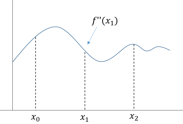
Consider at x₁. What if the change of slope (second derivative) is the same between two lines — the line from x₀ to x₁, and line from x₁ to x₂?

Let a = f’’(x₀), b = f’’(x₁) and c= f’’(x₂) be unknown constants, and ∆₀ = x₁−x₀. Suppose we have following equality:

• f’’(x) = Aa + Bb ∀x ∈ [x₀, x₁]
• f’’(x) = ℬb + Cc ∀x ∈ [x₁, x₂]

where A = (x₁−x) / (x₁−x₀), B = (x−x₀) / (x₁−x₀), ℬ = (x₂−x) / (x₂−x₁) and C = (x−x₁) / (x₂−x₁).

When we are starting at an arbitrary point “x” on the line between x₀ and x₁, we will get f’’(x₁) as we move to the point x₁. Similarly, if we are at point “x” that is between x₁ to x₂, we also obtain f’’(x₁) as we move to point x₁.

Next, we can build on the equality: ∀x ∈ [x₀, x₁]

As shown in above derivation, f(x) is a cubic function.

We can claim that f(x) is a cubic function just given that its second derivative is Aa + Bb, which means f ′′′(x) is a constant. Notice that the values of f(x₀) and f(x₁) are observed, so we can substitute them for finding the letters C and D.

Consider (2)−(1):

Then, we substitute this C into the formula of the first derivative as follows.

where

Notice that

also

Thus

Therefore

is the first derivative (Mr. Opengate).

Next, we want to take the integration. Consider

Thus, after taking integration on the first derivative, we have:

it follows that

In other words,

where (3)-(4) is

Finally, we have

where

We want to find this function f(x), so we need the values of a and b. We have assumed them to be unknown constants, now let us find their values.

Recall the latest formula for the first derivative becomes:

with a = f’’(x₀) and b = f’’(x₁). What we are going to do is to link two lines at the common knot. We have been talking about things happening in two points x₀ and x₁. Now, suppose f (xᵢ₋₁), f (xᵢ) and f (xᵢ₊₁) are observed. Consider ∀x ∈ [xᵢ₋₁, xᵢ]

and similarly ∀x ∈ [xᵢ, xᵢ₊₁]

At the intersection point xᵢ of these two functions, they should be the same in terms of their location (C⁰ continuity) and their velocity, i.e., first-order derivative (C¹ continuity). After that, we let f’(xᵢ⁻) be the slope at xᵢ on the line joining xᵢ₋₁ and xᵢ, and let f’(xᵢ⁺) be the slope at xᵢ on the line joining xᵢ and xᵢ₊₁ so that we suppose:

Notice that the first second derivation is M₀ and the last is Mₙ, we can put all the equations with i = 1, 2, …, n-1 into a matrix expression as follows.

There are n+1 unknown second derivatives: M₀ . . . Mₙ. In other words, we need two more constraints to solve for all Mᵢ.

The not-a-knot condition implies that the second and second-last points (in our case the points: x₁ and xₙ₋₁) are not knots. At the beginning of the whole function joining all the points universally, from x₀ to x₂ the function is a line without any knot at x₁ in the sense that it is C³-continuous at x₁ (Jeffrey Chasnov). What happening at the second last point xₙ₋₁ is just the same.

As we have mentioned C³ continuity, we need to consider the third derivative. Recall we have the format:

Note that the expression of the third derivative is ∀x ∈ [xᵢ, xᵢ₊₁], and the second derivative f’’(xᵢ) is an unknown constant. Similarly ∀x ∈ [xᵢ₋₁, xᵢ] we have:

The not-a-knot condition only applies to x₁ and xₙ₋₁. That’s, for i = 1, n − 1 we have the C³ continuity as follows.

Applying Not-a-knot Condition

For all points, recall that for all i = 1 … n−1

where

First of all, we consider when i = 1 the general equation becomes

and the not-a-knot condition is

consider (5) + ∆₁λ₁(6):

We assume ∆₀ ≠ ∆₁ for the time being, otherwise 𝜆₀ and D₀ are not defined.

Next, we consider the case when i = n−1 as follows.

and the not-a-knot is

consider (7) + ∆ₙ₋₂(1 − λₙ₋₁)(8):

Same as before, we assume ∆ₙ₋₂ ≠ ∆ₙ₋₁ otherwise 𝜆ₙ and Dₙ are not defined.

Eventually, we have the fully fledged system as follows (Antony Jameson).

Let’s see if we can build the tri-diagonal system when data are evenly spaced at the head and tail such that ∆₀ = ∆₁ and ∆ₙ₋₂ = ∆ₙ₋₁.

We can substitute M₀ = 2M₁ − M₂ (from not-a-knot condition) into the equation in the first row: (1-𝜆₁)M₀ + 2M₁ + 𝜆₁M₂ = D₁ in order to obtain M₁ = D₁/3. Therefore, the not-a-knot condition becomes

and recall that first two rows and last two rows are:

Substitute the not-a-knot into (9) and (11) we have

We need a 2 before M₀ and Mₙ because later you will see there is also a 2 before each Mᵢ in the system of equations.

𝜆₀ is definite if 𝜆₁ ≠ 1 and 𝜆ₙ is definite if 𝜆ₙ₋₁ ≠ 0. Notice that ∆₀ = ∆₁ and ∆ₙ₋₂ = ∆ₙ₋₁ in this case, thus 𝜆₁ = ∆₁ / (∆₀+∆₁) = 1/2 and 𝜆ₙ₋₁ = 1/2 as well. Therefore, 𝜆₀ and 𝜆ₙ are well defined.

Recall again the first two rows and last two rows:

consider (10) − (1 − λ₂)(9)/2

consider (12) − λₙ₋₂(11)/2

Therefore,

and M₁ and Mₙ₋₁ are given by the not-a-knot condition directly. Solving all Mᵢ in the tri-diagonal system, we can find all the cubic functions between knots, and the whole cubic spline is found.

TriDiagonal Matrix Algorithm (TDMA)

The method of solving a tri-diagonal system below is provided by (A. Salih). Today, we are going see how it works on solving cubic spline from scatter points. Consider solving the vector u in following equation:

for i = 1…N.

The last line comes from realising that in the first row, u₁ can be expressed in u₂, then recursively in the second row u₂ can be expressed in u₃. Note that with the equation in the first row and the expression of uᵢ we have:

Next, substitute uᵢ₋₁ (expressed using P and Q) into the expression of dᵢ as follows.

Note that the red line is in the same form as the previous red line. Also, note that P₁ and Q₁ are known, and additionally their values can be found by substituting a₁ = 0 into the expression of Pᵢ and Qᵢ above.

If we force c_N to be zero, with the equation of Pᵢ

The last entry in the vector u needs to be Q_N. So, starting from P₁ and Q₁, we get P₂ and Q₂, then recursively all Pᵢ and Qᵢ are computed. After Q_N is computed, u_N is known. According to above red formula, all uᵢ can be computed recursively as well.

This is what we get!

Now it comes to the most interesting part of this article. We are going to merge above knowledge in the crystal ball of maths!

Suppose ∆₀ ≠ ∆₁ and ∆ₙ₋₂ ≠ ∆ₙ₋₁. Then, for i = 1 … n+1 let

If we change the index — for i = 0 … n

where

are known, so all pᵢ and qᵢ are known. Now, consider

Notice that

Therefore, after Mₙ = qₙ is computed, we can find all Mᵢ.

Since all second derivatives are computed, the sub-functions of the spline between each pair of points are solved. This means f’(xᵢ⁻) = f’(xᵢ⁺) and not-a-knot condition are observed. Also, by the design in the very first place of this article that the function is expressed deliberately in forms such as f’’(x) = Aa + Bb, the whole spline created is also C²-continuous.

And we are done!

We finally get to the end of this long article. Let me know if there is any mistake I have made. Thank you for your reading and see you in my next article! 👍👍👍

References:

• Article: 🔖A. Salih, Tridiagonal Matrix Algorithm 🔖Mr. Opengate, 三次樣條插值 Cubic spline interpolation 🔖Antony Jameson, Cubic Splines (p.5)
• YouTube: 🔖Jeffrey Chasnov, Cubic Spline Interpolation (Part B) | Lecture 45 | Numerical Methods for Engineers (4:05) 🔖Freya Holmér, The Continuity of Splines (15:31)