Advanced Ray Tracer: Part 4

In this part, I implemented texture mapping, Perlin noise, normal mapping, bump mapping. I also added bump mapping with the generated Perlin noise and a cool procedural checkerboard texture. All of these features help us add more realism and help us create more versatile scenes. I expected this part to be easier than the first three as it required less algorithmic complexity (kind of ignored the given hint about the part) which was my mistake. This was probably the most challenging part for me but I think I managed.

All images seen in the post are rendered by my raytracer. In this post, I will try to go from the simpler concepts to the more advanced ones while also explaining the ideas in depth. This time, I did not run time tests as the images generally have low sample counts. So let’s begin!

Galactica Static — Texture Mapping, Bump Mapping

Texture Mapping

Texture mapping is the concept of putting a previously creates image on an object. This might be something like putting a wood texture on a wooden table or putting a painting texture on a paper. The ideas are limitless here. You can even use only textures to determine the shading coefficients of objects, although this would be inefficient and quite weird. So we generally use this technique to broaden the stuff we can do with our ray tracer and render images with anything displayed or written on them that would be extremely difficult or impossible to generate by our own.

Background

I believe the first thing I should get out of the way is the preliminary of this whole process of mapping something onto a mesh or sphere. The main thing to consider first is the range we use as our texture coordinates. We usually map our textures in the [0, 1] range. The textures are 2D images so we use a 2D coordinate system denotex by (u, v).

Our textures are given to us in some kind of image format that we read. The issue here is finding out where to look when a ray hits an object and that object has a texture assigned to it. The spherical case is quite simple as we usually use angles to parameterize the mesh and get (u, v) values (each between 0 and 1) to find out where to look in the given texture. In most cases, we would consider out texture’s corners to be (0, 0), (0, 1), (1, 0) and (1, 1) so our (u, v) values fit them.

But how can we find such a mapping when we have a complex object with a texture like the spaceship in the galactica scene above? In our case, every vertex that came with the object also includes a texture coordinate associated with it. ın the simplest case, these textures coordinates will be between 0 and 1 as I mentioned earlier. And the texture we use for the spaceship looks something like this:

Galactica Spaceship — Texture atlas

This is called a texture atlas. So combining these we can deduce that someone actually parameterized this mesh for us beforehand and painted the textures for it knowing this parameterization. Mesh parameterization is actually a huge area in and of itself. I am currently working on a project related to this topic and planning on blogging it too. You can check it out in the blog page in the following weeks.

The main idea you should keep in mind right now is:

• Only we parameterize the spherical objects
• Someone previously parameterized and gave us the coordinates of where the vertices of the mesh lie on the texture
• The texture values we want to read might not exactly need to be where the vertices are. Only vertices’ parameterizations are known. We need to come up with a way to handle when a ray hits on the inside of a triangle

So having the idea of what we get as input.

Texture Mapping Spheres

The spherical case requires us to think of two angles: theta and phi. These represent the angles the point we want to get the parameterization of makes according to the sphere. If you think of a 3 dimensional space with a sphere centered at the origin, the phi angle could be the angle between the point’s projection on the x, z plane and the theta angle could be the angle between the point’s projection on the y, z plane:

Sphere Texture Mapping — Lecture Notes by AO Akyüz

We already know where the ray hit so we know the x, y and z coordinates. So we get the theta and phi angles in radians, but the ranges for them are different. You can see from the image above that the phi angle spans a whole circle from both sides, while theta spans only one side: one spans form [- pi , pi] and the other [0, pi].

Mapping these onto the [0, 1] range is actually quite easy. We can just add pi to -phi and divide it by 2pi to get the u coordinate. We can also just divide theta by pi to get the v coordinate. I think the reason we use -phi is about the orientation we want to utilize the texture and later the normal orientation we use: right handed or left handed.

So we get the u and v coordinates with in between our desired range.

Texture Mapping Triangles

Texture mapping triangles is easier. We are already (but only) given the (u, v) values of the vertices. But when a ray hits a triangle, we need to get its (u, v) by using these values. We can use barycentric coordinates to achieve this. You might remember this from the first part of the series. We can get a weighted average of the texture coordinates of the vertices by using this. Let’s recall:

Barycentric Coordinates — Lecture Notes by AO Akyüz

Here we would normally find the intersected point’s coordinates by using this formula:

Barycentric Coordinates — Lecture Notes by AO Akyüz

In this case, we will use this for the texture coordinates and all will be done:

Texture Mapping Barycentric Coordinates — Lecture Notes by AO Akyüz

So having these u and v values, we can move onto actually reading data from the textures. But there might be a middle step here that we need to stop by.

Tiling

For larger surfaces we would like to add textures to, we might refrain from only 1 texture that goes through the whole surface. This would cause distortions in the texture’s look. Instead, we would want to repeat the texture on the surface as big as is. Some texture coordinates are given to us in the scenes in larger values than 1. This is the case where tiling happens. If our found u and v values are bigger than 1, we take the integer floor and subtract it from the u and v values. For example if the u value is 3.30, subtracting the floor would be: 3.30–3.00 = 0.30. The same could be done with the v values. This is like a mod function and it helps us repeat the texture over the surface.

Tiling — Lecture Notes by AO Akyüz

The problem here might be that the repetition look clearly in some cases, but this is not something we need to focus on right now.

Interpolation Strategies

Having the u and v values, we can convert them to image space coordinates ranging from [0, image width] and [0, image height]. We can do this simply by multiplying the u with the image width and the v with the image height. Let’s call these values i and j.

The issue here is that our textures are in image format and we can not directly access texel(‘texture element’, data in a simple texture image pixel) values using floating point numbers, only integers. Our point likely lies in between several integer values and therefore pixels we could read from. We can follow multiple paths here.

Nearest Neighbor

The first thing we could do is, we could just round the i and j values and get the nearest integers to them. Then we can read from the image using these. This would obviously be really fast, but not give the smoothest results as we only round and do not interpolate.

Bilinear Interpolation

Bilinear interpolation is a better way. We just get the average of the four closest neighbors. You can think of a pixel falling in between 4 texel center points anyways so this is pretty easy to visualize:

Bilinear Interpolation — Lecture Notes by AO Akyüz

Trilinear Interpolation

Trilinear interpolation is much more complicated than the first 2 ways. It was first talked about by Lance Williams in his 1983 paper ‘Pyramidial Parametrics’. I read the paper and tried to understand the concept more in depth by doing some extra research.

This approach requires mipmaps to function. Mipmaps are progressively smaller versions of a texture. An example from the paper:

Mip map of the flexible NYIT Test Frog — Williams, L. (1983). Pyramidal Parametrics.

Why the paper’s name include pyramidial is that, Williams thought about layering these mipmap levels on top of each other and sampled from the neighboring two at the same time. You can see a representation of this here:

Mipmap and Mip hierarchy representation — CMU Computer Graphics Lecture Notes

When researching more, one of the clearest definitions was this from a blog post:

The visible transition between the MIP maps can finally be countered with trilinear interpolation. Where bilinear interpolation interpolated in two dimensions by blending four pixels, trilinear interpolates in three dimensions. The extra dimension is a blend between two MIP maps. The number of memory operations is now eight: four pixels in each of the two MIP maps that we interpolate between. — Bikker, J. Optimizing Trilinear Interpolation.

I will not talk about it much more as I did not implement this. I actually never planned to, just wanted to gain insight and give some to the reader. You can check out the sources I will add at the end.

Utilizing Read Data

So we are close to the end of our process. We read RGB values from the textures at this point and can utilize them in our shading process to give our objects some extra color. There are a couple of things we can directly do. We can put these RGB values in the [0, 1] range and use them as our diffuse reflectance coefficient, specular reflectance coefficient or blend them with each other.

Finally, time to see some cool rendering results that you can compare approaches:

Plane Nearest Neighbor

Plane Bilinear

Sphere Nearest Bilinear

As you can see, my results also show that bilinear interpolation works much better than the nearest neighbor approach. It would be cool to also compare with trilinear interpolation…

Here are other examples with a more ‘real world’ use case:

Cube Wall— Replacing kd

Wood Box — Replacing kd and ks

In the Wood Box case, we also replace the specular reflectance coefficient reading a texture to dampen the excessive reflection of light on the wooden surface. Here is how it looks without replacing ks:

Wood Box No Specular — Only replacing kd

The texture we use here to replace the specular reflectance coefficient looks like this:

Wood Box Specular Texture

What is cool with this is that it removes specular reflectance from the wooden part while keeping it in the metal areas. I think this is a cool trick. There is another really cool trick we can do to add some background.

Background Textures

You can guess what we will do here quite easily. Our near plane that we send rays through is also a rectangular surface and we can associate a texture to it and approach it like a plane with z = infinity. If our rays do not hit any object, we normally return the background color, in this case, we will return the color of the texture, according to the point the ray goes from in the near plane. This is how we get the space background in the galactica scenes:

Galactica Static — Background Texture

So we are done with the main texture mapping part. The procedures I mentioned here will also be used for normal and bump mapping. The difference will be what we will do with the values we read.

But first, let’s talk about procedural textures. Procedural textures are ones that are generated on the fly without using texture images. We will look at the approaches I implemented in this part and their use cases.

Perlin Noise

Procedural textures can be generated in many ways. The simplest ones might be the ones that are generated using trigonometric functions or checkerboard which we will talk about later. What these textures lack is they do not look natural at all. To make procedural textures look more natural, we need to add some randomness, but too much would also look quite unnatural as it will turn into extreme noise. One idea could be to hold random values for each integer (x, y, z) coordinate in our space and interpolate between these points with trilinear interpolation to get the controlled random value. But this would occupy too much memory as we would need a 3D lattice that is bigger than the whole scene. Ken Perlin created a solution for this problem in his paper ‘An Image Synthesizer’, published in 1985. Here are the steps to his solution in 3D:

• Associate 8 random gradient vectors at grid corners
• Compute the vectors from the corners to the desired point
• Compute the dot product of each vector with the corresponding gradient vector
• Compute the contribution of each corner based on the distance of the point to the corners
• Finally: 2 ways to visualize

I believe this is easy to follow except the last 2 parts. To compute the contribution of each corner, we use this function:

Perlin Noise Interpolation — Lecture Notes by AO Akyüz

Then we can calculate weights by:

Perlin Noise Weights —Lecture Notes by AO Akyüz

These weights are for 2D here, need to add 4 more and all of them should also have the z values.

Before moving onto the final visualization part, I want to touch on the first part: associating 8 random gradient vectors at grid corners.

Random Gradient Vectors

As I mentioned, the crucial part of this algorithm is that we do not have to store a 3D grid as large as the scene itself. What we do instead is, we pseudorandomly choose gradient vectors using a hash function. In this case, when we want to calculate the noise for a point, no matter how many times we do it, we will get the same gradient vectors for each point.

Here, a pseudo-random permutation table and pseudo-random unit-length gradient vectors are used in the hash function. We can see more about the implementation and how it was improved by Perlin in his paper ‘Improving Noise’ published in 2002:

Deficincies in Original Algorithm — Perlin, K. Improving Noise. 2002.

As you can see, they first used another function for the interpolation. In this paper, Perlin proposed a new one (similar to ours):

New Interpolation Function — Perlin, K. Improving Noise. 2002.

He also mentioned a problem about there being directional bias here:

Directional Bias Problem — Perlin, K. Improving Noise. 2002.

He proposed a new set of gradient vectors to keep to solve this problem:

Unit Length Gradient Vectors— Perlin, K. Improving Noise. 2002.

So he concluded that the permutation table produced enough randomness and decided to go with a set of clearly defined unit vectors. I am not quite sure why the other approach would cause problems. Here is the last thing he does:

Padding to 16 — Perlin, K. Improving Noise. 2002.

I am not quite clear on why he does this either but this whole paper resembles AO Akyüz’s approach.

My Implementation

I read this paper after implmenting Perlin noise myself. I just wrote a simple hash function and my approach was really basic, I just multiplied the x, y and z values by some large numbers and added them up, then did a bitwise shift and XOR. I also used these 12 vectors and ones with the same magnitude, but only in the x, y and z directions. So I had 18 vectors, I just ran the hash function, took mod 18 and got the gradient vector. Then continued with the following steps. My approach worked just fine so I did not want to change it.

Having covered this part, we can move onto the visualization.

Final Noise

Upto the final part, our noise value is typically in the range of [-1, 1]. We can do 2 things here. We can just add 1 and divide by 2, this would be a typical way to put it between 0 and 1. We can also take the absolute value of the noise which would increase contrast.

Here are my results:

Cube Perlin

Sphere Perlin

We can also change the scale of our Perlin noise texture, which would make it fuller:

Sphere Perlin Scale

Multi-Octave Perlin Noise

One last thing we can do is introduce a multiple octave Perlin noise. Here is the formula we can follow:

Multi-Octave Perlin Noise — Part 4 Notes by AO Akyüz

In this formula, K is the number of octaves. By default this value is 1 as n is our noise function and we only run it as is only once. If the number of octaves is bigger than one, the frequency is doubled and the weight is halved. s is the total accumulated noise.

This is actually easy to visualize. Higher frequency would mean finely detailed or repeated noise, lower would be much broader. Here, we go from lower to higher frequency while decreasing the weight. This means that the broader noise octaves we get will be much more appearent and we will add the high frequency noise with little weight so it will be less distinct. We can get marble, smoke and cloud-like results with this approach.

Here is an example using multiple octaves:

Dragon — 7 octaves — by Ramazan Tokay

This looks great in my opinion and is the coolest scene I have rendered so far. Many thanks to Ramazan!

So being done with Perlin noise, we can move onto the second procedural texture.

Checkerboard Pattern

This was by far the easiest part. I do not want to stay on this for a long time at it is extremely simple. I just followed this pseudocode:

Checkerboard Pseudocode — Part 4 Notes by AO Akyüz

And tried the texture with one of the box scenes:

Cube Wall Checkerboard — Problematic

There was a lot of noise so I added small epsilon values to the function and all was fine:

Cube Wall Checkerboard

There are 2 small white dots near the corner but I think that is just okay at this point. Let’s move onto the next part!

Normal Mapping

Now we move onto another territory where we will try to make it look like the object’s geometry changes. What would be best for this is displacement mapping. With normal and bump mapping we will not get self shadows. On the other hand displacement mapping provides a more realistic look including self shadows by actually changing the geometry. In this part we will only change the normals that we use in shading to make it look like objects have some geometric features when they really do not.

Normal mapping is where we read the texture value and use that value as our new normal. We need to figure out how to represent normals in the range [-1, 1] using the 0–255 values we read from the image. To map them to 3D directions, the following formula can be used:

Reading Normal Values — Lecture Notes by AO Akyüz

Then we need to normalize. Getting this done, we should move on to the most crucial point.

Triangle Normal Mapping

Normals in these textures are defined in the canonical tangent space of the surface. What you might think of is, the texture has its own space, and its own 3 orthogonal vectors, we need them to fit the surface’s corresponding vectors, so we need to transform them. We know in the texture space we have U and V, now we also have W as the normal. In the real tangent space of the surface we have (T, B, N) which are tangent, bitangent and normal vectors which correspond to U, V and W. Explaining all the steps to find the transformation matrix would take too long, so I will give some formulas:

Finding Tangent and Bitangent Vectors — Lecture Notes by AO Akyüz

In this equation, T and B are the tangent and bitangent vectors and that is what we want to find. E1 and E2 are two edges that share a point on the triangle we hit. delta u and delta v are the differences in the u and v vectors of E1 and E2. After getting the tangent and bitangent vectors, we need to normalize them. Then we can calculate (bitangent x tangent) to get the new normal.

Sphere Normal Mapping

With spheres, we will get our (u, v) values exactly the same way we did in texture mapping. Then we will plug the u and v values back into the x, y and z values as such:

Plugging (u, v) into x,y and z — Lecture Notes by AO Akyüz

So here we denote x, y and z in terms of u and v. Right now, we can take x, y and z’s partial derivatives with respect to u and v. This would give us how much the point’s coordinate changes as u and v change. And this operation would exactly give us the tangent and bitangent vectors.

Partial Derivatives to find T and B — Lecture Notes by AO Akyüz

This operation results in the following:

Partial Derivatives to find T and B — Lecture Notes by AO Akyüz

After finding the T and B again, we can normalize them and take their cross product to find a new N.

So at this point, we have T, B and N vectors for the triangular and the spherical cases. How can we make use of them?

Final Steps

As we have the T, B and N vectors, we can now find our final new normal by turning this into a transformation matrix and transforming our initially found and normalized (x, y, z) normal vector:

Finding the new normal — Lecture Notes by AO Akyüz

So at this point, everything should be done. Here are some cool results with normal mapping:

Cube Cushion with Normal Mapping

Cube Waves

Cube Wall with Normal Mapping

Brick Wall with Normal Mapping

To illustrate this further, I can remove the coloring in the last 2 textures to only display the normal mapping part:

Cube Wall with Only Normal Mapping

Brick Wall with Only Normal Mapping

So this part looked like a success. Although I had some issues regarding implementing the formula. I wrote some stuff wrong and I captured one of the wrong inputs beforehand:

Cube Waves Problematic

This was fixed quite easily as I found a mistake in one of the formulas.

Having this done, we can move onto bump mapping.

Bump Mapping

Unlike normal mapping, bump mapping does not completely change the normals of the surface. It only perturbs the existing normals using a height function it reads from the texture. I think this was the trickiest part. We will rely more on partial derivatives here and it is kind of math heavy.

First of all, we will define our bumped surface as:

Bumped Surface — Lecture Notes by AO Akyüz

Here p is the point, h is the height function and n is the normal. Then we can find our new normal as we did with the bitangent and tangent vectors: by taking the cross product of partial derivatives:

New normal — Lecture Notes by AO Akyüz

So we need to find the partial derivatives first. By using the chain rule, we can find:

Bumped Surface Partial Derivatives — Lecture Notes by AO Akyüz

Again the whole idea here is that we want to find the bumped surface’s function and how it changes as u and v changes. Then we can get the cross product of the changes in these 2 directions and get our new normal.

As you might remember, the red circled parts are the tangent and bitangent vectors respectively. And the green circled are the partial derivatives of the height function. We can define a height function roughly by putting the read RGB values into the [0, 1] range and then adding them up. We can also divide by 3 to also put it in the [0, 1] range to add normality. We can find the derivatives of the height function by using the method of forward differences:

Forward Differences — Lecture Notes by AO Akyüz

delta u and delta v can be picked as 1 / image_width and 1 / image_height. But I think this roughly corresponds to stepping into the next texel in each direction so getting the next texel directly could work. Then we will multiply this with our normal and add up with the tangent and bitangent vectors for each case.

The computation of the last uncircled part of our surface equation is really complex and adds little to the overall surface so we will ignore it. I wanted to illustrate the idea:

Here is our main setup. We will only look at the difference in the direction of the u vector as drawing also with v would be difficult.

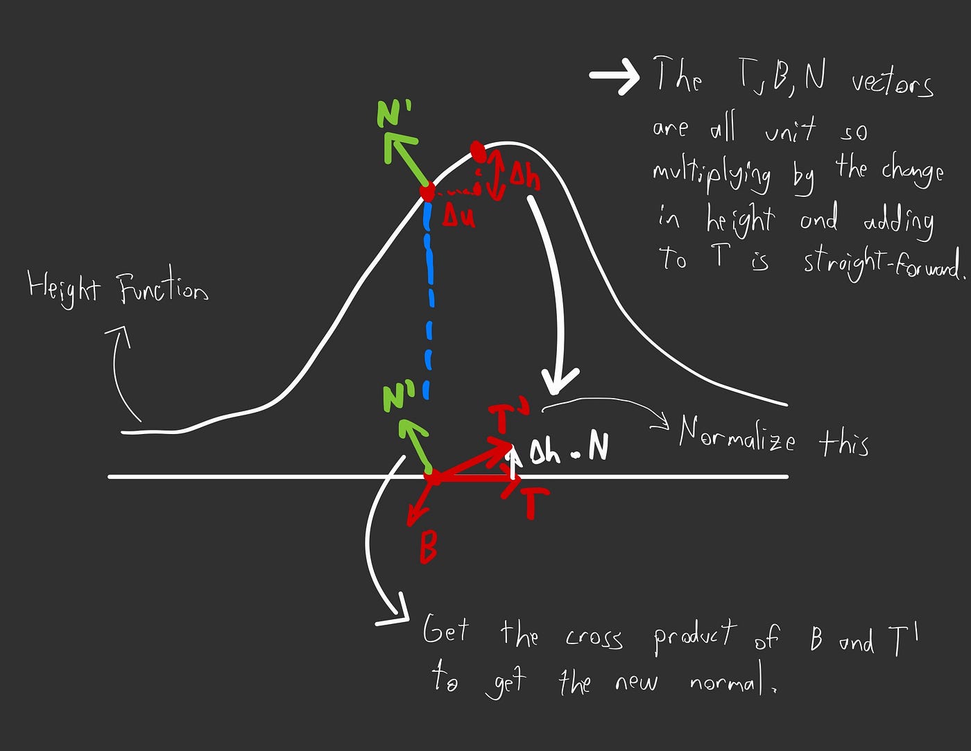
I think this is a good and clear way of getting the basic idea.

Finally, I want to briefly summarize what we do here:

• Get the tangent and bitangent vectors that correspond to the u and v vectors in the texture the same as in normal mapping.
• Read from the texture and put the read RGB values in a determined height function.
• Take the height function’s partial derivatives which corresponds to how much height changes when we continue in the u and v directions and multiply that with the normal.
• Sum up the tangent vector which represents the change in the real surface when we go in the u direction with the multiplication of the normal and the change in the height function when we go in the u direction. And same with the bitangent vector and the v direction.
• This whole process will perturb our tangent and bitangent vectors in the direction of the surface normal according to the height function(which would be varying according to the texture).
• We will take the cross product of these perturbed vectors to get our final perturbed normal.

After doing all of this, I saw bumps but they were not that correct:

Sphere Bump Test — Problematic

Turns out I forgot to multiply with pi in one of the formulas. This was extremely irritating as it took me long hours to find. Again the perturbations were not that appearent in my case so I multiplied with a constant to exeggerate them. I think the problem might be that I missed some normalization somewhere. But the results look pretty cool right now:

Wood Box All — Only Bump Mapping

Wood Box All

Sphere No Bump — Bump

Sphere No Bump — Just Bump

Bump mapping also works with transformations:

Bump Mapping Transformed

Bump Mapping Transformed — Only Bump Mapping

I actually had a problem with these scene before:

Bump Mapping Transformed — Problem

This was due to the very small scaling of a plane. I just increased the bounding box epsilons a little bit than before and it was solved.

Here is the previous galactica scene and a showcase of how we can combine with the features from the last part:

Galactica Static — Uses Bump Mapping

Galactica Dynamic — Bump Mapping and Motion Blur

This was another extremely cool scene. Here is another one where the surface texture coordinates are not in the range of 0 to 1 but 0 to 4. In this case we just tile the existing texture, something I mentioned at the beginning of the post:

Killeroo Bump Walls

Here is another scene with transformations that showcases the features we have implemented upto this point (it’s a texture modified version of the ellipsoids scene from part 2):

Ellipsoids Texture

But there remains one last thing we will do which is bump mapping with Perlin noise.

Bump Mapping with Perlin Noise

In this case we also follow the same main route as the original bump mapping case. We follow the same formula to get qv and qu and take the cross product. After simplifying the equation, we get this:

New Normal in Bump Mapping with Perlin Noise — Lecture Notes by AO Akyüz

The component we subtract from the normal is called the surface gradient. In our case, Perlin noise is a scalar field and its gradient is the vector that points along the greatest change of this scalar field. The surface gradient is this vector’s projection on the tangent plane.

Getting Surface Gradient — Lecture Notes by AO Akyüz

We can find the surface gradient after calculating the gradient vector as follows:

Calculating the Gradient Vector — Lecture Notes by AO Akyüz

All of these ideas utilizing partial derivatives and gradient vectors could be hard for you to understand if you have not used them for a while. I suggest you watch this 5 minute video to get an idea and read the whole process from the beginning.

[embed]

After implementing all of this, I had these results:

Sphere Perlin Bump

Cube Perlin Bump

As you can see, for the linear and absolute value approaches of Perlin noise, we get different results as expected here. The linear approach creates a tennis ball-like result in the spherical case. The absolute value approach looks more brainy.

These look great but I have some remaining issues in this part.

Problems

I have problems in 2 scenes in this part so the streak of going faultlessly has kind of ended. I added all of the features I should have but I believe I have the same problem of parsing the mytap and veach_ajar scenes. These scenes have .ply files that include the (u, v) coordinates next to the (x, y, z). I think I have a problem with reading these u and v values as the mytap scene’s texture looks skewed.

My Tap — 4 Samples — Problematic

I also can not render the veach_ajar scene as I can not do the first parsing of the scene, it does not continue to the rendering stage. I was not sure on why it would not work so decided to check the scenes from the prior parts to see if I broke something, but scenes from part 2 and part 3 were all okay. I will try to find the source of this issue.

I can’t decide if having these types of problems like parsing is better or worse than the actual subject related issues, nevertheless this infuriated me. I tried to solve it at the last day for a couple of hours but could not find the root. I did not want to break anything further as only 2 hours were left and decided to stop there.

Some Notes

I also stumbled upon something called parallax mapping in the book Real Time Rendering, written by Akenine-Möller and his collegues. In the book, what parallax mapping is good for and what it adds is written very clearly. Here it why it is used.

A problem wiwth bump and normal mapping is that the bumps never shift location with the view angle, nor ever block each other. If you look along a real brick wall, for example, at some angle you will not see the mortar between the bricks. A bump map of the wall will never show this type of occlusion, as it merely varies the normal. It would be better to gave bumps actually affect which location on the surface is rendered at each pixel. — Akenine-Möller et. al. 2018. pp. 214- 215.

I would want to look more into this and explain it here but I do not have much time at this point and this post will almost get past 5000 words. Nevertheless it seems to be a cool approach.

Conclusion

This part did not have algorithmic complexity, but it was quite hard and the workload was higher than usual. Some concepts were really interesting and I spent hours trying to learn more stuff in depth. I woultd consider this part a success not from the success of the rendered scenes but broadening my perspective on the world of computer graphics so I am quite happy with it. In the next part we will work on new light source types and HDR tonemapping. See you then!

References

Akenine-Möller, T., Haines, E., Hoffman, N., Pesce, A., Iwanicki, M., & Hillaire S. (2018). Real-time rendering (4th ed.). A K Peters/CRC Press.

Akyüz, A.O. Lecture Slides from CENG795 Advanced Ray Tracing. Middle East Technical University

Bikker, J. (2020). Optimizing trilinear interpolation. Jacco’s Blog. Retrieved from https://jacco.ompf2.com/2020/04/10/optimizing-trilinear-interpolation/

Carnegie Mellon University. (2016). Computer graphics: Texture mapping [Lecture slides]. Retrieved from https://www.cs.cmu.edu/afs/cs/academic/class/15462-s16/www/lec_slides/07_texture.pdf

Perlin, K. (1985). An image synthesizer. ACM SIGGRAPH 1985 Conference Proceedings, 19(3), 287–296. ACM. https://doi.org/10.1145/325165.325247

Perlin, K. (2002). Improving noise. ACM SIGGRAPH 2002 Conference Proceedings, 681–682. ACM. https://doi.org/10.1145/566570.566636

Physics Videos by Eugene Khutoryansky. (2016, January 9). Gradients and Partial Derivatives [Video]. YouTube. https://www.youtube.com/watch?v=GkB4vW16QHI