Decoding LLMs — Part 2: A Step-by-Step Journey Into the Mind of Modern AI

In Part 1, we built something powerful a rich, contextual representation of the sentence “How are you.” The encoder did its job beautifully. Every word is understood, every relationship mapped, every position locked in.

But here’s the thing we still haven’t said a single word in Hindi.

That’s the decoder’s job. And it’s a fascinating one.

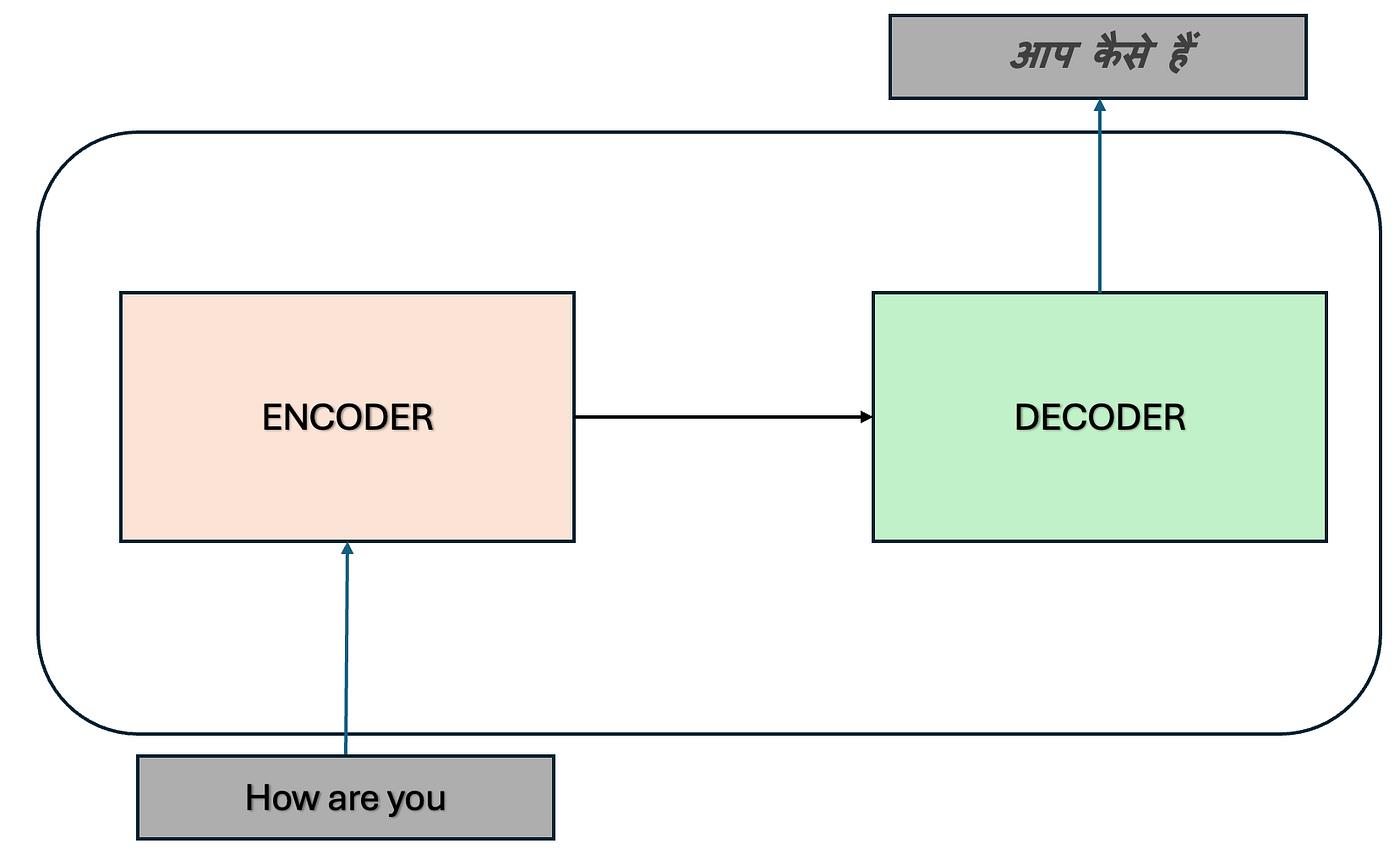
Figure 1: Encoder and Decoder of the Transformer

Just like the encoder stack, the decoder is not a single block either it is a stack of N decoders, each layer refining the output generation further. And just like the encoder, each decoder block has its own internal machinery that we’ll pull apart piece by piece.

But before we understand what happens inside the decoder let’s first understand what goes into it.

Step 1: Input to the Decoder

Before we understand how the decoder works, let’s take a step back and look at the training data itself.

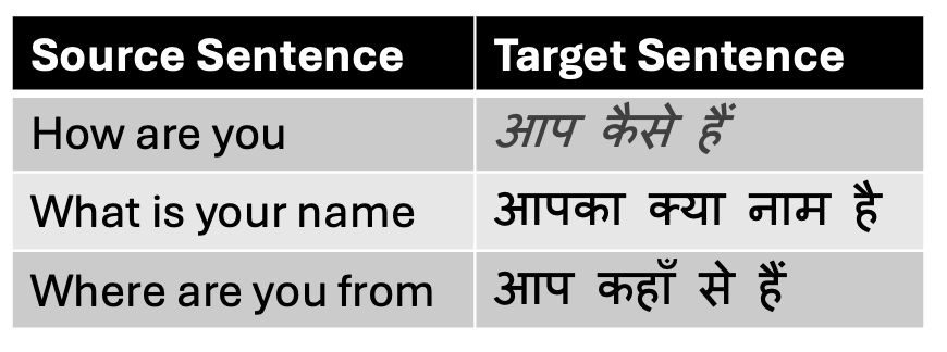
Figure 2: Sample Training Data

The table tells a simple but important story for every Source Sentence fed into the encoder, there is a corresponding Target Sentence that the decoder is expected to produce. The encoder’s job is to deeply understand the source. The decoder’s job is to generate the target one word at a time.

For our example:

• Encoder input → “How are you”
• Expected decoder output → “आप कैसे हैं”

Once the encoder has finished processing the source sentence and produced its rich contextual representation, the baton is passed. The decoder now takes the stage using the encoder’s output alongside its own input to generate the translation word by word.

But what exactly is the decoder’s own input? That’s where it gets interesting.

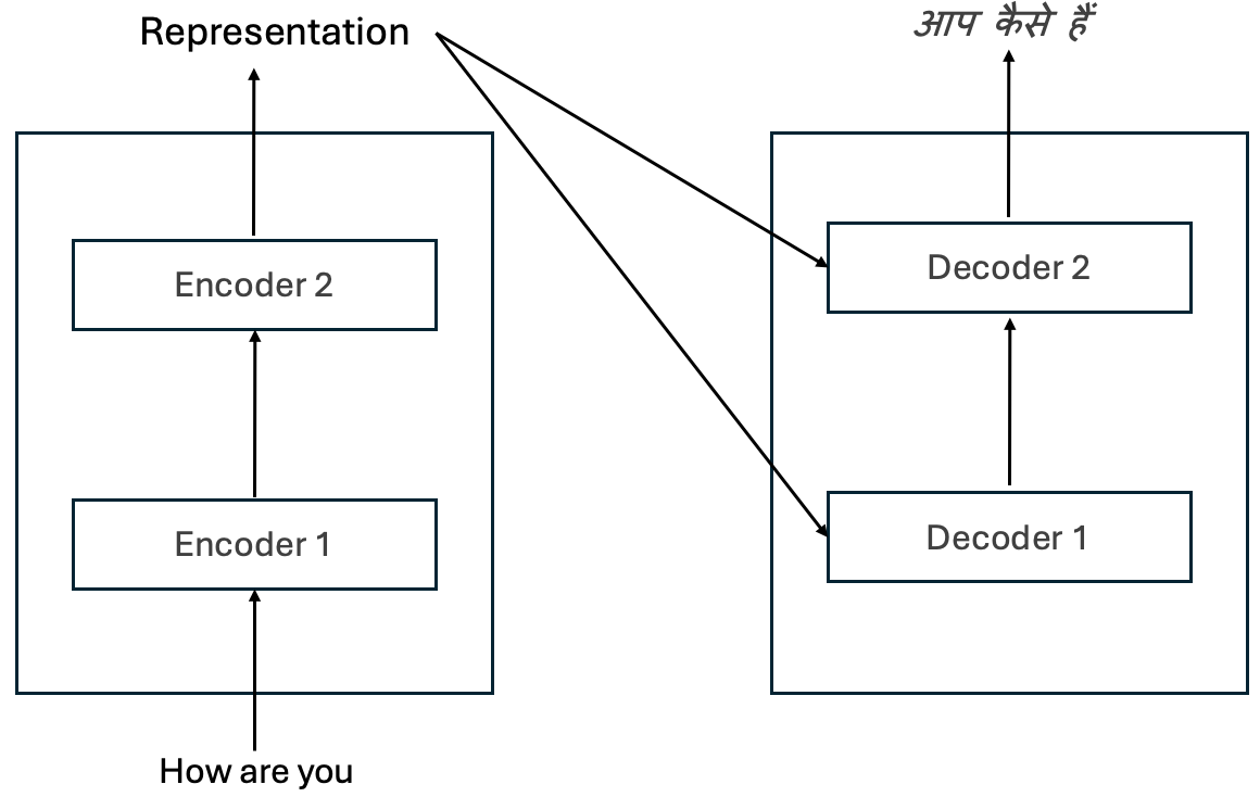
Figure 3: Encoder–Decoder Workflow for English-to-Hindi Translation

The diagram reveals something important, the encoder representation doesn’t just flow into the first decoder and stop there. It flows into every decoder layer in the stack. Here is exactly how the information travels:

• Decoder 1 receives two inputs — the target sentence (<SOS> आप कैसे हैं) and the encoder representation of “How are you”
• Decoder 2 also receives two inputs — the output from Decoder 1 and once again the same encoder representation

This is a crucial detail, the encoder output is not consumed once and discarded. It is a shared reference that every decoder layer consults independently, ensuring the full context of the source sentence is available at every stage of generation.

Think of it like a translator who keeps glancing back at the original English sentence not just once at the beginning, but at every step of writing the Hindi translation.

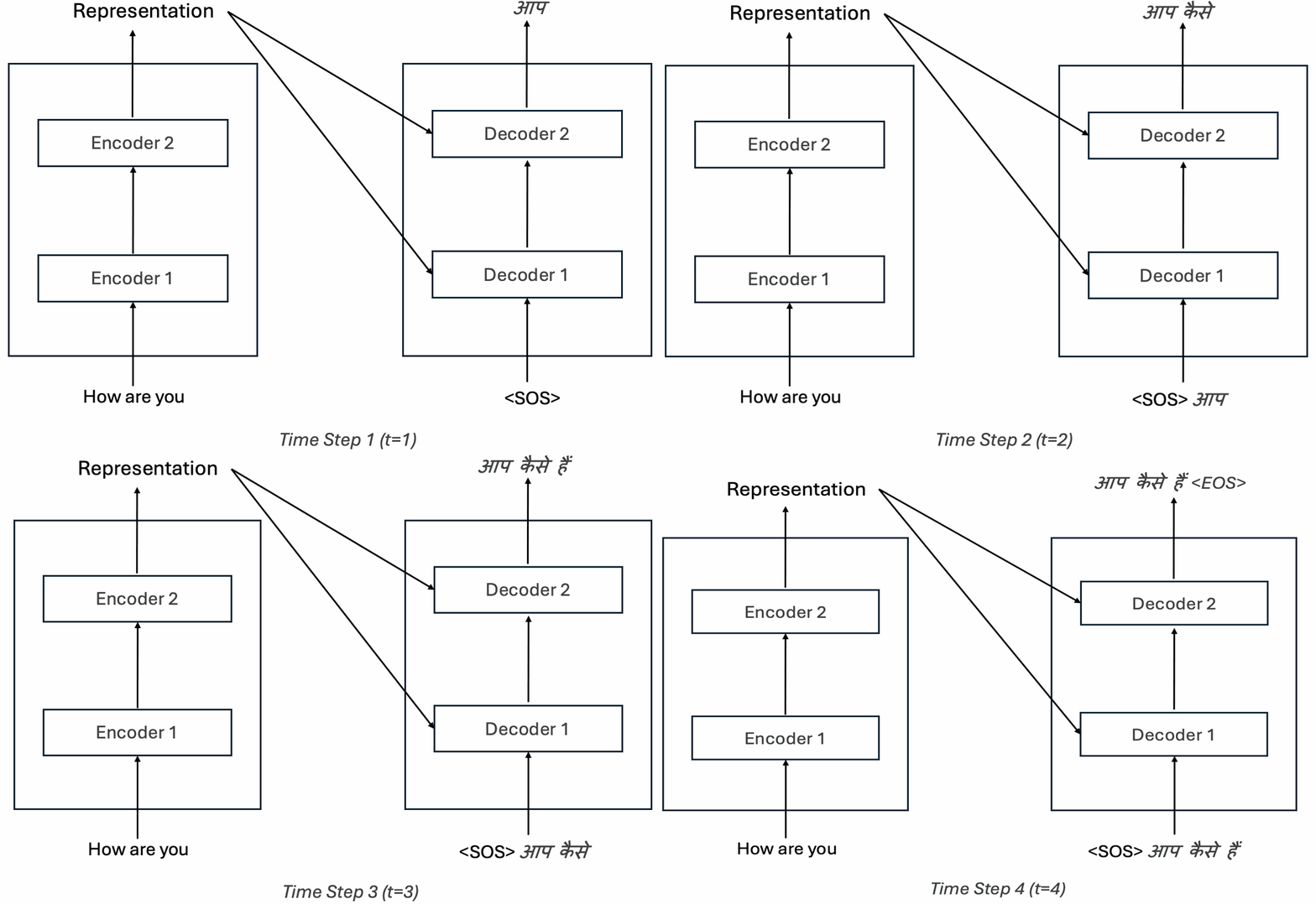
Figure 4: Visualization of Word-by-Word Input Processing Across Time Steps

The GIF walks us through the decoder in action and it’s more intuitive than it looks. Let’s follow it step by step:

Time Step 1 — The Starting Signal The decoder receives a single token as its first input the special <SOS> (Start of Sentence) tag. This is the decoder’s cue to begin. Using the <SOS> token alongside the encoder’s representation of “How are you”, the decoder generates its first Hindi word “आप.”

Time Step 2 — Building on the Previous Output The decoder now receives two things the <SOS> token and the word it just generated “आप.” Using this growing context it predicts the next word “कैसे.”

Time Step 3 — The Sequence Grows The same pattern continues <SOS>, “आप”, “कैसे” are all fed in together and the decoder predicts “हैं”.

Final Step — Knowing When to Stop Once the full translation is generated, the decoder produces a special <EOS> (End of Sentence) tag its way of saying “I’m done.” The translation is complete.

This process of feeding previously generated tokens back into the decoder at each step is called autoregressive generation the decoder builds its answer one word at a time, each prediction informed by everything it has generated so far.

Now, just like the encoder, before feeding this sequence into the decoder we need to give every token two pieces of information what it means and where it stands. But first things first we need to tokenize our input.

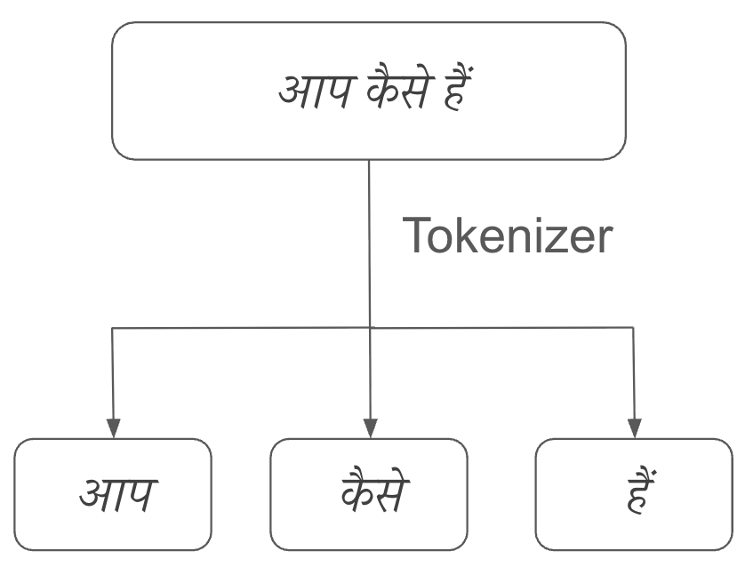
Figure 5: Sentence Tokenization into Words

Once the input is tokenized, the next step is identical to what we did in the encoder generating positional encodings for every token in the decoder’s input sequence.

Figure 6: Decoder Input Representations with Positional Embeddings

Just like before even dimensions use sine, odd dimensions use cosine, and every token gets a unique positional fingerprint that tells the model exactly where it sits in the sequence.

The only difference here is the sequence itself, instead of encoding the English source sentence, we are now encoding the Hindi target sequence <SOS> आप कैसे हैं.

Final Decoder Input = Token Embeddings + Positional Encodings

With our decoder input fully prepared, let’s zoom out and see how everything fits together so far.

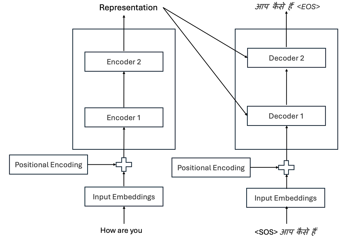
Figure 7: How Information Flows from Encoder to Decoder and Within the Decoder

During training, instead of letting the decoder use its own predicted output as the next input, we feed it the correct target sentence from the start — all at once. This technique is called Teacher Forcing and it makes training significantly faster and more stable.

But here is where the decoder’s architecture diverges from the encoder for the first time.

In the encoder, the output of Token Embeddings + Positional Encodings flows directly into Multi-Head Attention. The decoder does something different it routes the same combined input into a Masked Multi-Head Attention layer instead.

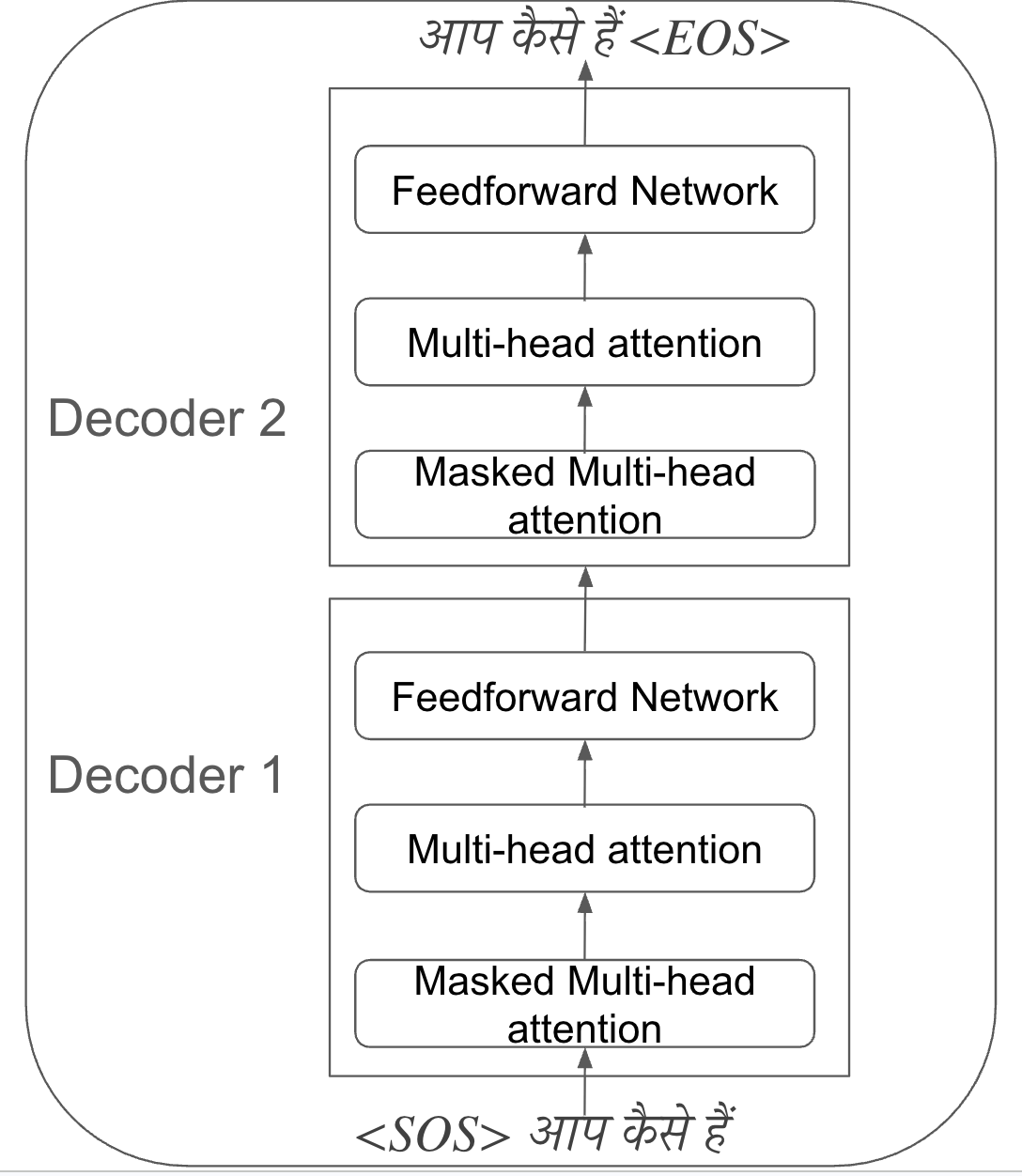
Figure 8: Key Components of the Transformer Decoder

The mask is the critical difference. Since we are feeding the entire target sentence at once during training, the model could theoretically peek at future words while predicting the current one, which would be cheating. The mask prevents exactly this by blocking each token from attending to any word that comes after it.

“आप” can only see → <SOS> ✅ “आप” cannot see → कैसे, हैं ❌

This forces the decoder to predict each word using only what has come before exactly as it would during inference when generating word by word.

Masked Multi Head Attention

During training we have a luxury that doesn’t exist at inference time we already know the correct target sentence. This means we can feed the entire sequence <SOS> आप कैसे हैं to the decoder all at once rather than waiting for each word to be generated step by step.

But this creates a problem.

If the decoder can see the entire target sentence at once what is stopping it from simply looking ahead and cheating? During inference the model has no future words to peek at it generates word by word, each prediction based only on what came before. If we train without any restrictions, the model never learns to work under real conditions.

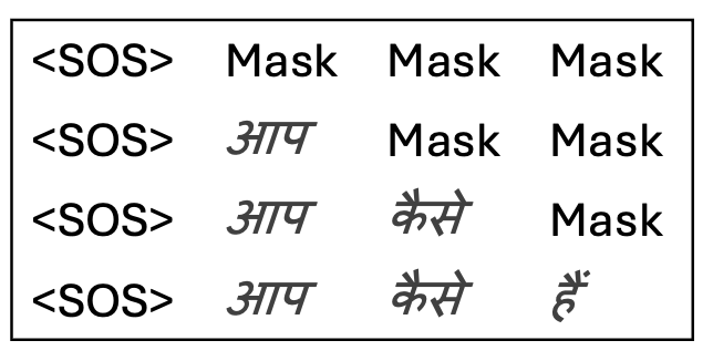
Figure 9: How Masking is Applied to Input Sequences

The above figure makes the pattern clear each token can only see what came before it. Future tokens are completely hidden, replaced by a Mask.

Here is exactly how this masking is applied inside the attention mechanism. The first two steps are identical to regular multi-head attention:

Step 1 — Compute Q × Kᵀ Multiply the Query matrix with the transpose of the Key matrix to get the raw attention scores.

Step 2 — Scale Divide the scores by √dk to keep the values stable.

Step 3 — Apply the Mask Before softmax, every future position is replaced with -infinity. This is the critical step that makes masking work when softmax is applied to -infinity, it produces exactly zero. Future words don’t just get less attention they get no attention at all.

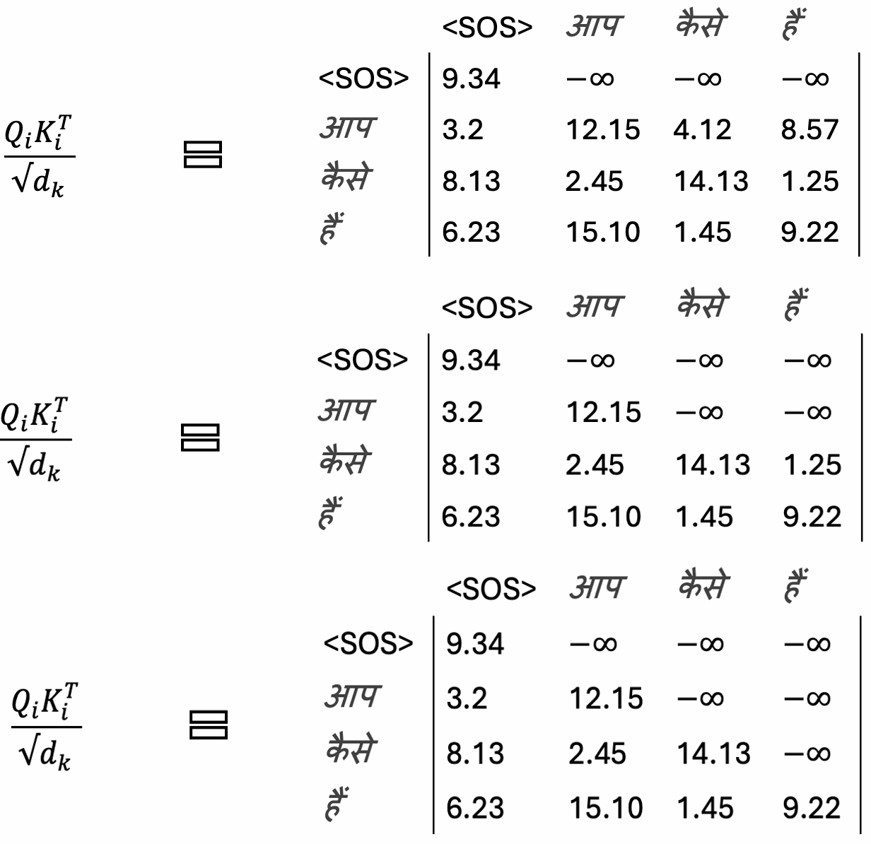
Figure 10: Visualization of −∞ Masking Applied at Each Time Step

Step 4 — Softmax Apply softmax to convert the remaining scores into attention weights between 0 and 1.

Step 5 — Multiply with Value Matrix Multiply the attention weights with the Value matrix to get the final self-attention output for each token.

Once all attention heads have computed their outputs independently, we concatenate them into a single matrix and multiply by the learned weight matrix W exactly as we did in the encoder. This produces the final masked attention output, which is then passed forward to the next layer of the decoder.

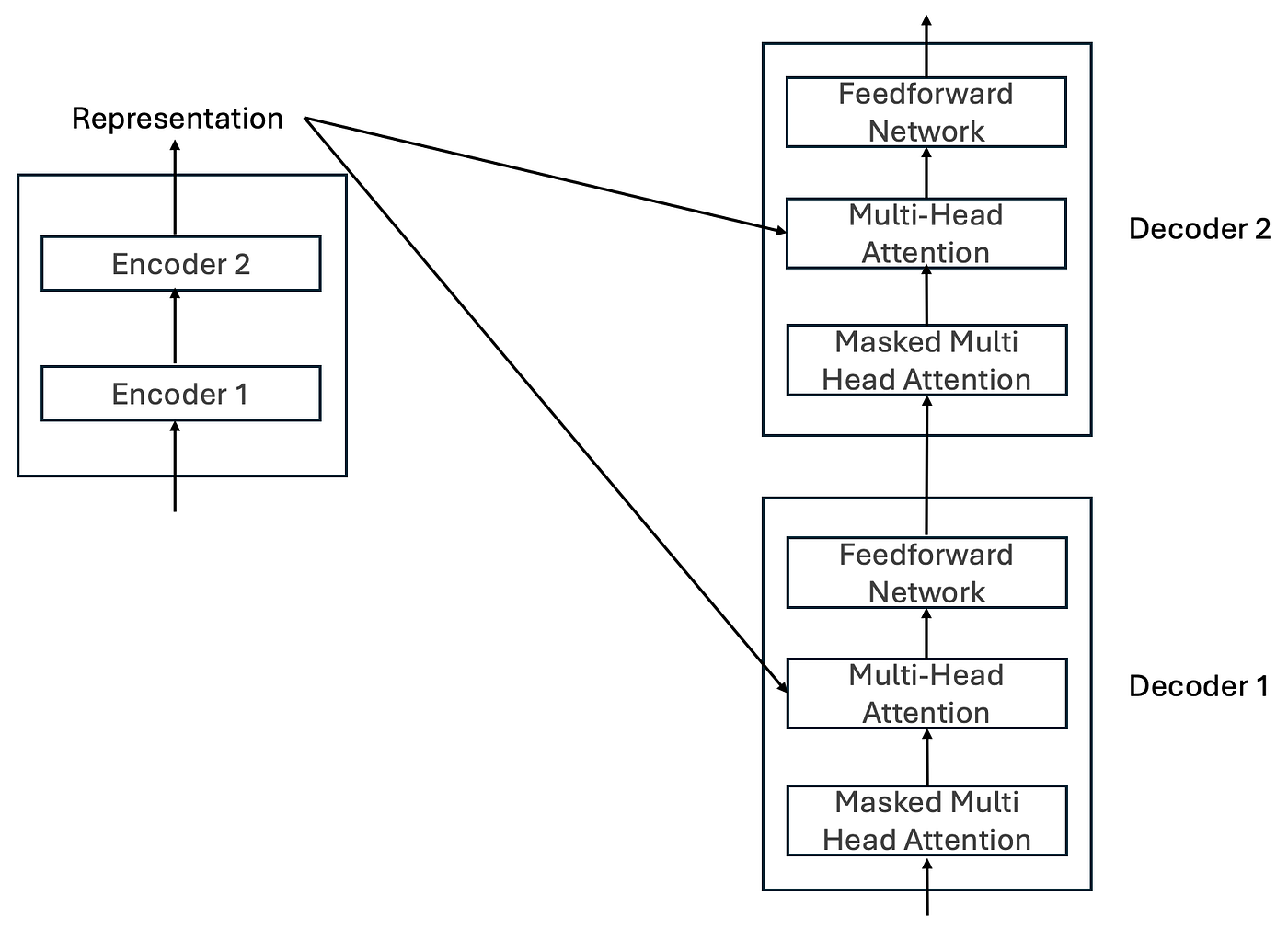
Figure 11: How Information Flows Through the Encoder–Decoder Architecture with Decoder Blocks

And this is where something remarkable happens.

Looking at the diagram, notice that the next layer Multi-Head Attention receives not one but two inputs:

• The output from the Masked Multi-Head Attention layer below it — the decoder’s own contextual understanding of the target sequence so far
• The encoder representation — the rich contextual understanding of the source sentence “How are you”

This is no longer self-attention where a sequence attends to itself. This is Cross-Attention the moment where the encoder and decoder finally meet. The decoder stops looking inward and starts asking the encoder a very specific question:

“Given everything I have generated so far — which parts of the English sentence should I focus on to generate the next Hindi word?”

The answer to that question is what drives the translation forward.

Multi-Head Attention — The Same Mechanism, A Different Source

In the encoder, all three matrices Query, Key and Value came from the same sequence. The decoder’s cross-attention breaks that pattern with one important twist.

• Query (Q) → derived from M — the masked attention output from the previous sublayer
• Key (K) and Value (V) → derived from R — the encoder representation

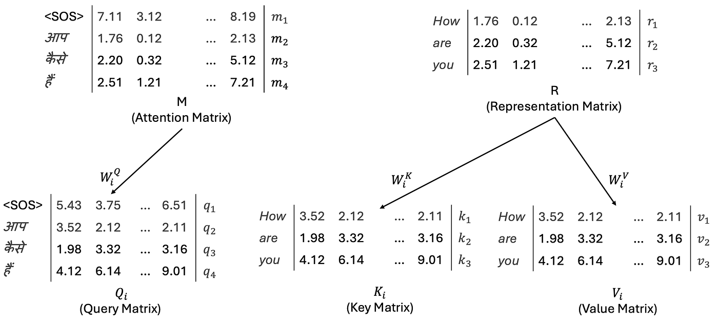
Figure 12: How Query, Key, and Value Matrices are Created in the Decoder for Multi-Head Attention

But why this specific split?

Think of it this way the Query is the question and the Key and Value are the answer.

Since Q comes from M it carries the decoder’s current understanding of the target sentence essentially asking “what Hindi word am I trying to generate right now?”

Since K and V come from R they carry the encoder’s complete understanding of the source sentence holding all the information about “How are you” ready to be retrieved.

Together they create a bridge the decoder’s question reaches into the encoder’s knowledge and pulls out exactly what it needs.

Once Q, K and V are established, the remaining steps follow the exact same self-attention process we covered in Part 1 scaling, softmax and multiplying with the Value matrix producing our final attention matrix Z.

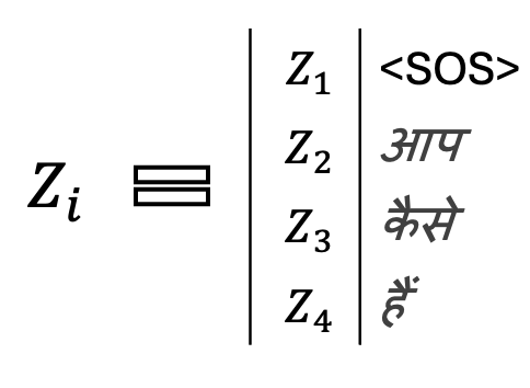
Figure 13: Attention Output Vectors Corresponding to Each Token

What Does Z Actually Represent?

Z is not just another attention matrix. At this point every decoder token carries something remarkable a blended representation of both languages simultaneously.

Figure 14: Attention Matrix Showing Alignment Between Input and Target Tokens

Each Hindi token now knows:

• Its own meaning and position from the masked self-attention
• Which English words to focus on from cross-attention with the encoder

This is the moment where translation truly happens not at the output, not at the softmax, but right here inside Z, where “आप” learns it belongs with “How” and “कैसे” learns it belongs with “are.”

But Z alone is not the final output of cross-attention. There is one more step that makes the decoder’s multi-head attention fundamentally different from the encoder’s.

The attention output of each token is multiplied with the Value matrix derived from the encoder representation R. This step is what allows the model to go beyond just knowing which English words to focus on it now extracts the actual content of those words and blends it into the decoder’s representation.

Figure 15: Cross-Attention Output Computed Using Attention Weights and Value Matrix

In other words Z told the decoder where to look. The Value matrix tells it what to take.

Together they produce something neither could alone a representation of each Hindi token that is simultaneously grounded in the target language and informed by the source. The decoder is no longer working in isolation. It has the full weight of the encoder’s understanding behind every single prediction.

Once all attention heads have independently computed their cross-attention outputs we concatenate them into a single matrix and multiply by the learned weight matrix W collapsing multiple perspectives into one unified multi-head attention output, ready to be passed to the next layer.

Now is a good moment to step back and formally introduce the term we have been building towards throughout this entire section Cross-Attention.

Cross-attention is simply the mechanism where:

• Query (Q) → comes from the decoder
• Key (K) and Value (V) → come from the encoder

The simplest way to remember the distinction:

Self-attention talks to itself. Cross-attention talks to someone else.

• Self-attention in encoder → “How” understands its relationship with “are” and “you”
• Self-attention in decoder → “आप” understands its relationship with “कैसे” and “हैं”
• Cross-attention in decoder → “आप” understands its relationship with “How”, “are” and “you”

This is the bridge between two languages the mechanism that allows the decoder to generate each Hindi word with a full understanding of the entire English sentence behind it.

Feedforward Network & Add Norm — The Final Decoder Layers

The next sublayer in the decoder is the Feedforward Network identical in structure to the encoder’s. Two dense layers with a ReLU activation in between, processing each token’s representation independently to add further depth before passing it forward.

Following the feedforward network, we once again apply the Add & Norm layer exactly as we did in the encoder. The residual connection adds the sublayer’s input back to its output, and layer normalisation stabilises the values row-wise before moving to the next step.

At this point one full decoder block is complete. In practice this entire block — Masked Multi-Head Attention, Cross-Attention, Feedforward Network and two Add & Norm layers is stacked N times, each layer refining the representation further.

From Representation to Words — The Linear & Softmax Layers

Once the final decoder layer has produced its output, we are still not quite done. The decoder’s output is a vector a dense numerical representation. To turn that into an actual Hindi word we need two final steps:

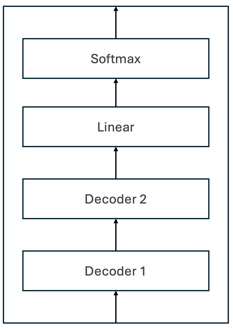
Figure 16: Post-Decoder Processing with Linear and Softmax Layers

• Linear Layer — projects the decoder output into a vector of size equal to the entire target vocabulary. Each position in this vector corresponds to one possible word in Hindi
• Softmax Layer — converts these scores into probabilities between 0 and 1 that sum to 1. The word with the highest probability is selected as the predicted output token

For our example — the model looks at every Hindi word it has ever seen during training and asks “which word most likely comes next?” The softmax output tells it with “आप” scoring highest at time step 1, “कैसे” at time step 2 and so on until <EOS> signals the end.

Let’s make this concrete with our example.

Suppose our entire target vocabulary consists of just three words:

Vocabulary = [आप, कैसे, हैं]

The linear layer produces a logit vector of size 3 one score per word in the vocabulary.

Now suppose the decoder has received <SOS> and “आप” as its input and needs to predict the next word. The output from the topmost decoder is fed into the linear layer which returns:

logits = [38,60,45]

Applying softmax converts these raw scores into probabilities. The highest probability sits at index 1 and looking that up in our vocabulary gives us “कैसे” exactly the correct next word in our translation.

“कैसे” is added to the output sequence and the process continues one word at a time until <EOS> is generated and the translation is complete.

Putting It All Together

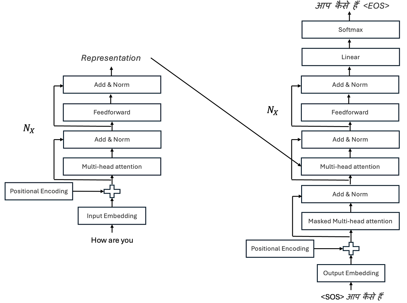
Figure 17: End-to-End Transformer Architecture for English-to-Hindi Translation (Single Encoder and Decoder)

Above is the complete Transformer architecture for our English to Hindi translation use case and take a moment to appreciate how far we’ve come.

What started as three simple words “How are you” went through an remarkable journey:

• Tokenization & Embeddings — words became vectors
• Positional Encodings — vectors gained a sense of order
• Masked Multi-Head Attention — the decoder learned to understand the target sequence without peeking ahead
• Cross-Attention — the encoder and decoder finally met, aligning English words with their Hindi counterparts
• Feedforward Network & Add Norm — representations were refined and stabilised
• Linear & Softmax — vectors became probabilities, probabilities became words

And the output? “आप कैसे हैं” three Hindi words that carry the full meaning, context and structure of the original English sentence.

This is the Transformer. Not magic just elegant mathematics, applied with extraordinary precision.

Every GPT, every BERT, every Gemini you use today traces its roots back to this architecture — to one paper, one idea, and one mechanism that changed everything: Attention Is All You Need.

This was Part 2 of Decoding LLMs. In Part 1 we built the encoder. In Part 2 we built the decoder. Together they form the complete picture of how a Transformer thinks, reads and speaks.

References Used: -

Vaswani, A., et al. (2017). Attention Is All You Need. Google Brain. https://arxiv.org/abs/1706.03762

Devlin, J. (2021). Getting Started with Google BERT. Packt Publishing.

OpenAI. (2024). ChatGPT (GPT-4). https://chat.openai.com

Anthropic. (2024). Claude. https://claude.ai