The Hidden Statistics Behind Your Daily Phone Activity

In today’s digital world, people check their phones countless times, yet their usage patterns are not truly random. Continuous probability distributions help analyze this behavior by revealing hidden patterns in screen-time data. For example, they can model how long users wait between notifications or how much time they spend scrolling. These methods go beyond simple averages to show deeper trends in user activity. As a result, they provide a scientific way to understand how people interact with technology.

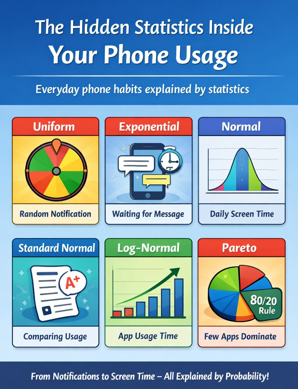
Turning Everyday Phone Habits into Statistical Insights

The Case Study

Rahul’s phone records his activity for 30 days. The data collected includes:

• Notification times
• waiting time between messages
• Daily screen usage hours
• App usage duration
• Comparison with friends
• App popularity

We analyze this same dataset from different statistical perspectives.

What is Continuous Probability Distribution ?

Continuous probability describes the likelihood of a variable that can take any value within a range, where probabilities are calculated for intervals rather than exact values.

Examples:

• Height of a person — can be 170.1 cm, 170.12 cm, etc.
• Time taken to finish a race — could be 9.5 s, 9.53 s, 9.531 s.
• Temperature of a city — may be 30.2°C, 30.25°C, etc.

A valid continuous distribution must:

• Never go below zero
• Total area must be 1
• Probabilities are calculated using integrals over ranges

Types Of Continuous Probability Distribution:

• Uniform
• Exponential
• Normal
• Standard Normal
• Log Normal
• Pareto

1. Uniform Distribution:

Uniform Probability Distribution

A continuous uniform distribution is a probability distribution in which a continuous random variable has an equal probability density for all values within a specified interval, meaning no value in the range is more likely to occur than another.

Formulae for the Continuous Probability Distribution

Imagine a mobile app sends notifications to users between 2:00 PM and 3:00 PM. The app’s algorithm ensures that every minute within this 1-hour window has an equal chance of sending a notification.

Why Uniform Distribution?

• Each time point in the interval [2: 00, 3: 00]is equally likely.
• No particular minute is favored over another.
• This randomness ensures fairness and avoids notification clustering.

Program to find the mean & Variance

Program to represent the visualization

Visualization of Uniform continuous probability Distribution

2.Exponential Distribution:

Exponential Probability Distribution

The Exponential Probability Distribution is a continuous probability distribution that describes the time between independent events that occur at a constant average rate.

Formulae For Exponential Probability Distribution

Suppose your smartphone receives notifications (messages, app alerts, emails) at a roughly constant average rate throughout the day.

Let

• X = time (in minutes) between two consecutive notifications
• λ = average notification rate per minute

Then X follows an Exponential Distribution:

• Mathemetical Representation : X∼Exponential(λ)

If your phone gets 3 notifications per minute on average:

• λ = 3
• Mean waiting time = 1 / λ = 1 / 3 minute ≈ 20 seconds

So on average, you wait about 20 seconds for the next notification.

Program to find Mean & Variance

Program to Represent the Visualization

Visualization of Exponential Probability Distribution

3.Normal Distribution:

Normal Probability Distribution

A Normal distribution is a continuous probability distribution that is symmetric about its mean, showing that values near the mean occur more frequently than values far from it. It is also called the Gaussian distribution.

Formulae for Normal Probability Distribution

If you measure daily phone usage of thousands of people:

• Most users spend around the average time (e.g., 3–4 hrs).
• Very few use it extremely little or excessively.
• This pattern also approximates a normal distribution

Properties:

• Mean = Median = Mode = μ
• Symmetrical bell shape
• Total area under curve = 1

Program to find Mean & Variance

Program to Represent the Visualization

Visualization of Normal Continuous Probability Distribution

4.Standard Normal:

Standard Normal Probability Distribution

The standard normal distribution is a special case of the normal (Gaussian) distribution that has a mean (μ) equal to 0 and a standard deviation (σ) equal to 1. It is a continuous probability distribution that describes how values of a variable are distributed around the mean in a symmetric, bell-shaped curve.

Mathematically, a random variable Z follows a standard normal distribution if: 𝑍 = (𝑋 − 𝜇) / 𝜎

where

• X = original variable
• μ = mean of the population
• σ = standard deviation

Formulae for Standard Normal Probability Distribution

Imagine a study measuring daily screen time (in hours) for 10,000 smartphone users.

• Average screen time (mean μ) = 5 hours
• Standard deviation (σ) = 1 hour

Researchers want to know how unusual a person’s usage is compared to others.

Program to Find Mean & Z-Score

Program to Represent the Visualization of Plots

Visualization of Standard Normal Continuous Distribution

5.Log Normal:

Log Normal Continuous Probability Distribution

A random variable X is said to follow a log-normal distribution if the natural logarithm of X is normally distributed. In other words:

If Y = ln(X) follows a normal distribution, then X follows a log-normal distribution.

Formulae for log Normal Continuous probability Distribution

Daily screen-time usage of smartphone users.

• Screen time is always positive (can’t be negative).
• Usage grows through multiplicative behavior:
• Notifications → open phone → watch video → open another app → time increases exponentially.
• Most people use phones for moderate time.
• A few users spend very long hours (gamers, streamers, binge watchers).

This creates a right-skewed distribution:

• Left side → many low/moderate users
• Right tail → few extreme users

Program to find Mean & Variance

Program to Represent the Visualization of Plots

Visualization of log-Normal Continuous Probability Distribution

6.Pareto Distribution:

The Pareto distribution is a continuous probability distribution used to model situations where a small number of events account for a large portion of the effect (often called the 80–20 rule). It describes phenomena with heavy tails, meaning extreme values occur more frequently than in normal distributions.

Formulae for pareto Distribution

The Pareto distribution is useful in analyzing mobile usage patterns because many phone-related behaviors follow a few-large, many-small pattern.

1. App Usage Time

• A small number of apps (≈20%) take most of your screen time (≈80%).
• Example: WhatsApp, YouTube, Instagram dominate usage while dozens of apps are rarely opened.

2. Data Consumption

• Few activities consume most mobile data:
• Video streaming
• Video calls
• Downloads
• Many other actions (texts, emails) use very little data.

Program to find Mean & Variance

Program to Represent the Visualization of Plots

Visualization of Pareto Continuous Probability Distribution

Special Case:

In phone analytics, special cases of the Pareto distribution describe whether usage is dominated by a few apps or evenly distributed, depending on the shape parameter α.

Conclusion:

In phone usage, continuous probability distributions help model measurable behaviors like screen time, data usage, and session length, showing how these values vary smoothly over time.

1. Normal Distribution Represents natural, symmetric data patterns (heights, marks). Most values cluster around the mean.

2. Binomial Distribution Models outcomes with two possibilities (success/failure) across fixed trials, such as correct answers in a test.

3. Poisson Distribution Used for counting rare events occurring in a fixed interval, like number of calls received per hour.

4. Exponential Distribution Describes waiting time between events, such as time between messages or arrivals.

5. Uniform Distribution All values in a range are equally likely, like random number generation.

6. Pareto Distribution Models unequal distributions where few items dominate most of the effect (80/20 rule), such as app usage or wealth.