Building a Simple RAG-Based Question-Answering System with Wikipedia

Retrieval-Augmented Generation, or RAG, has become one of the most common patterns in modern AI systems. It appears in chatbots, search tools, and question-answering products built on private knowledge bases. The reason is simple: people want language models to answer not only from what they learned during training, but also from specific documents that belong to a certain data collection.

This is where RAG becomes useful. A standard language model can generate fluent text, but it does not automatically know which external documents it should rely on. If the answer depends on constantly changing dataset, the model needs a way to access that information at runtime. RAG solves that problem by combining retrieval and generation in one pipeline. First, the system searches a document collection for relevant passages. Then it gives those passages to the language model as context and asks it to answer based on them.

In this post, we will build a simple version of that pattern. It will be a question-answering system based on Wikipedia. The goal is not to create a huge production platform, but to understand the core mechanics clearly. We will build a service where a user can ask a question and the system answers it using Wikipedia data.

What’s in this post

• Building a simple QA service based on existing language models
• Understanding the stages of RAG
• A code example

What’s not in this post

• Training language models
• Scaling the service for a large number of users

Wiki QA

We want a user to ask a question, search our own document collection for relevant text, and then generate an answer grounded in that text. In this project, the document collection is Wikipedia.

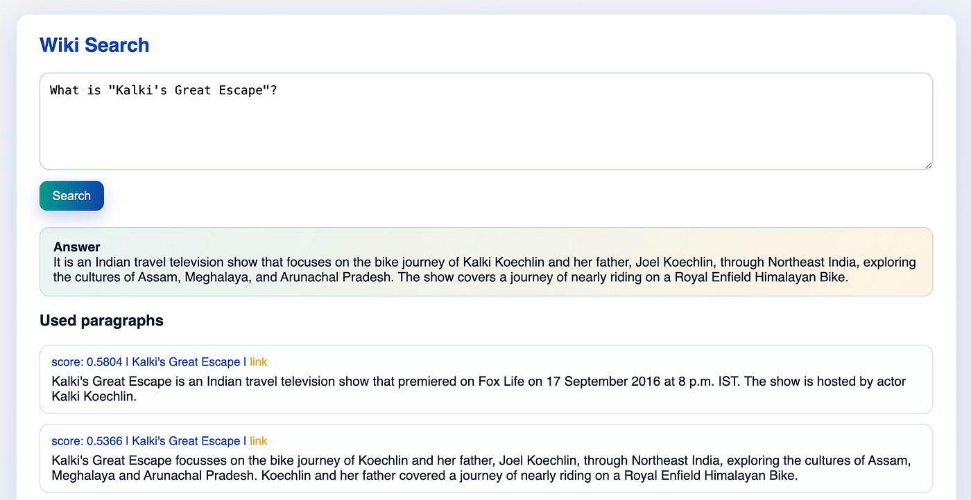
From the user’s point of view, the service is very simple. They open a web page, type a question into the input field, and send it. After that, the system returns two things on the same page: the generated answer and the text pieces that were used to produce that answer. The user can see not only the final response, but also the evidence behind it.

Pipeline

First, let’s look at the entire pipeline. We need to prepare the data for the retrieval stage. The system will search for an answer based on this data. To do this, we’ll take Wikipedia articles, break them down into small, meaningful chunks, and use a embedding model to represent them in vector space. We’ll build an HNSW index on the resulting vectors, which allows for fast search. Text paragraphs will be stored in SQLite database.

Now, when we receive a question from the user, we’ll also convert it into a vector and use the index to find nearby texts that will be used as candidates for finding the answer.

To generate the answer itself, another model will be used that was trained for this purpose. We’ll provide it with a special prompt and the candidates found in the previous step as input. The resulting answer will be displayed in the Flask service along with the candidates used to answer it. The whole code of project is here. Now let’s go into more detail about each step.

Whole RAG pipeline

Project Structure

WikiQA/
├── configs/
│   ├── access.yaml
│   ├── build_hnsw.yaml
│   └── service.yaml
├── data/
│   └── index/
│       └── wiki_hnsw/
│           ├── index.bin
│           ├── manifest.json
│           └── passages.sqlite3
├── src/
│   ├── api/
│   │   ├── __init__.py
│   │   ├── app.py
│   │   └── templates/
│   │       └── index.html
│   ├── retrieval/
│   │   ├── __init__.py
│   │   ├── build_hnsw.py
│   │   ├── hnsw_index.py
│   │   └── tools.py
│   └── __init__.py
├── .gitignore
├── README.md
└── requirements.txt

Before going into the methods, it helps to understand how the project is organized. The codebase is split into a retrieval part, an application part, configuration files, and the saved index artifacts.

The retrieval logic lives in src/retrieval/. The main file there is hnsw_index.py, which contains the HnswIndex class. This is the central class of the project. It knows how to build the index from the dataset, how to save and load the retrieval artifacts, how to search the HNSW index, and how to fetch retrieved passages from SQLite. The file build_hnsw.py is the command-line entrypoint for the build stage. The file tools.py contains helper utilities such as config loading and access-token reading.

The serving logic lives in src/api/. The file app.py contains the Flask application, the ServiceConfig class, the RAG orchestration class, and the AnswerGenerator class. This is the part of the project that turns the retriever and the generator into a working web application. The HTML template used by Flask is stored in index.html.

The configuration files live in configs/. The file build_hnsw.yaml controls the offline build stage. It contains dataset parameters, embedding model settings, paragraph chunking sizes, multi-processing settings, and HNSW parameters. The file service.yaml controls the online Flask service. It contains the path to the built index, the generation model name, the device, the number of retrieved candidates, and the answer length limit. The file access.yaml stores the Hugging Face access token when one is needed.

The generated retrieval artifacts are written into data/index/wiki_hnsw/. After the build stage, this directory contains the HNSW binary index, the SQLite database with stored passages, and the manifest file describing the built retriever.

Data Storage

The HnswIndex class will be responsible for structured storage and retrieval. Let’s build it step by step.

We start with a Wikipedia dataset: omarkamali/wikipedia-monthly. Each dataset row contains article text and metadata such as title and URL. During the offline build stage, the system reads each article and splits the article text into paragraph-sized chunks. We need this to control the context size for the generative model. Unfortunately, we couldn’t pass all Wikipedia data into our model — it has limited context capacity, and we also have time constraints when answering a user.

Step 1: Load the dataset

The dataset is loaded by HnswIndex._load_dataset:

@staticmethod
def _load_dataset(dataset_path: str, dataset_name: str | None, split: str):
    dataset = load_dataset(dataset_path, dataset_name, split=split)
    logging.info(
        "Loaded dataset '%s' (name=%s, split=%s) rows=%d",
        dataset_path,
        dataset_name,
        split,
        len(dataset),
    )
    return dataset

This method is simple, it keeps the data source configurable from build_hnsw.yaml. Let’s look at which parts of this config are useful right now:

dataset_path: omarkamali/wikipedia-monthly
dataset_name: latest.en  # Take only English articles for simplicity
split: train

At this point, the system has raw Wikipedia rows. Those rows are still too large to search directly, so the next step is chunking.

Step 2: Split article text into paragraphs

That logic lives in HnswIndex._split_paragraphs.

@staticmethod
def _split_paragraphs(
    text: str,
    min_paragraph_size: int,
    max_paragraph_size: int | None = None,
) -> List[str]:

    split_parts: List[str] = []
    for paragraph in re.split(r"\n{2,}", text):
        if len (paragraph) < min_paragraph_size:
            continue
        if len(paragraph) <= max_paragraph_size:
            split_parts.append(paragraph)
            continue
        split_parts.extend(
            paragraph[i : i + max_paragraph_size]
            for i in range(0, len(paragraph), max_paragraph_size)
        )
    return split_parts

This method does three things in order.

First, it uses re.split(r”\n{2,}”, text) to split article text on blank lines. That gives us paragraph-like chunks.

Second, it removes short chunks with min_paragraph_size. Very short fragments are often low-value for retrieval.

Third, if a paragraph is longer than max_paragraph_size, it slices that paragraph into fixed-size character segments. That means by the end of this step, one Wikipedia article has been turned into a list of paragraph-sized chunks ready for embedding.

Step 3: Load the embedding model

Now we need to convert chunks into dense embedding vectors using an embedding model.

In this project, we use google/embeddinggemma-300m. Architecturally, it is a transformer-based encoder-style model that converts text into dense vectors. Those vectors are useful because semantically similar texts should be close in vector space. That is exactly what retrieval needs. For example, if the user asks a question about planets near Earth, paragraphs about our Solar System should end up close to that query even if the wording is different.

For this task, embeddinggemma-300m has practical advantages. It is much smaller than very large general-purpose models, so it is easier to run on local hardware.

@staticmethod
def _load_model(
    model_name: str,
    model_device: str,
    access_token: str | None,
) -> tuple[SentenceTransformer, int]:

    model = SentenceTransformer(
        model_name,
        use_auth_token=access_token or None,
        model_kwargs={"torch_dtype": torch.float32},
        device=model_device,
    )
    dim = model.get_sentence_embedding_dimension()
    return model, dim

This method takes three input variables. model_name is the Hugging Face ID of the embedding model. model_device tells the loader whether the model should run on CPU or GPU. access_token is optional and is only needed if the model requires authentication.

The method returns two things: the loaded SentenceTransformer model and dim, the embedding dimension. That dimension is essential because HNSW must know the exact size of each stored vector.

Step 4: Create the HNSW index

Those vectors are inserted into an HNSW index so they can be searched efficiently later. The expected query complexity is O(log N), where N is the number of vectors.

HNSW, or Hierarchical Navigable Small World, is a graph-based index for approximate nearest neighbor search. Its main purpose is to find vectors that are close to a query vector without having to compare the query against every single vector in the dataset. The structure is built as a multilayer graph. Every data point is a node, and each node is connected to a limited number of neighboring nodes. The upper layers are sparse and help the search quickly move into the right region of the dataset, while the bottom layer is denser and is used to refine the search and find the final nearest candidates.

HNSW index

At the highest layer, the algorithm takes the current node and compares it with its neighbors. If one of the neighbors is closer to the query vector than the current node, the search moves to that neighbor. Then the same check is repeated again from the new position. In other words, the algorithm behaves greedily: at each step it tries to move to a node that improves the distance to the query. This process continues until no neighboring node is closer than the current one. At that moment, the algorithm assumes that it has reached a good local position in that layer.

The final work happens at the bottom layer, which is the densest layer and contains all indexed vectors. The algorithm begins from the entry node passed down from the layer above and places it into a priority structure. Then it repeatedly takes promising candidates, examines their neighbors, and adds better ones into the search frontier. A parameter called efSearch controls how wide this bottom-layer exploration becomes. If efSearch is small, the algorithm checks fewer candidates, so the search is faster but may miss some true nearest neighbors. If efSearch is larger, the algorithm explores more of the graph, which usually improves recall but also increases latency.

Search with HNSW index. The blue dots areindexed vectors, the pink dot is query vector and the light blue dot is the found neightbour

The vector search structure is built in HnswIndex._init_index:

@staticmethod
def _init_index(
    initial_index_size: int | None,
    space: str,
    ef_construction: int,
    m: int,
    ef_search: int,
    num_threads: int,
    dim: int,
) -> hnswlib.Index:

    index = hnswlib.Index(space=space, dim=dim)
    index.init_index(
        max_elements=initial_index_size,
        ef_construction=ef_construction,
        M=m,
    )
    index.set_ef(ef_search)
    index.set_num_threads(num_threads)
    return index

initial_index_size is the initial capacity of the index. space — name of the space, it can be one of “l2”, “ip” (inner product), or “cosine”, which is used in current project. ef_construction controls the size of the dynamic list for the nearest neighbors during index creation, and ef_search does the same during search. m defines the maximum number of outgoing connections in the graph. num_threads sets how many threads HNSW may use. dim is the embedding dimension.

At the same time, the original paragraph text and metadata are stored in a SQLite table under the same IDs used in the vector index. SQLite is useful here because it avoids keeping the full passage store in Python memory.

Step 5: Prepare SQLite storage

The paragraph text itself is not stored inside HNSW. It is stored in SQLite.

@staticmethod
def _init_sqlite_schema(sqlite_connection: sqlite3.Connection) -> None:
    sqlite_connection.execute(
        """
        CREATE TABLE IF NOT EXISTS passages (
            pid INTEGER PRIMARY KEY,
            row_id TEXT,
            url TEXT,
            title TEXT,
            paragraph_index INTEGER,
            paragraph TEXT
        )
        """
    )
    sqlite_connection.execute("CREATE INDEX IF NOT EXISTS idx_passages_pid ON passages(pid)")
    sqlite_connection.commit()

This method takes one input variable, sqlite_connection, which is the open SQLite database connection. It creates the passages table and an index on pid.

Each passage row stores the passage ID, the original row ID from the dataset, the source URL, the article title, the paragraph index inside the article, and the paragraph text. The design point here is that HNSW stores vectors and IDs, while SQLite stores the text behind those IDs.

Now that we’ve determined the data source, model, and storage location, let’s write the methods responsible for processing the dataset.

Step 6: Iterate over the dataset and process batches

The main indexing loop is HnswIndex._build_paragraph_index:

def _build_paragraph_index(
    self,
    dataset: Dataset,
    min_paragraph_size: int,
    max_paragraph_size: int | None,
    max_articles_to_process: int | None,
    batch_size: int,
    index_path: Path,
    manifest_path: Path,
    sqlite_path: Path,
) -> None:

    text_batch: List[str] = []
    meta_batch: List[dict] = []
    try:
        for row_idx, row in enumerate(tqdm(dataset, desc="Articles", unit="article")):
            if max_articles_to_process and row_idx > max_articles_to_process:
                break
            paragraphs = self._split_paragraphs(
                row["text"],
                min_paragraph_size,
                max_paragraph_size,
            )
            for paragraph_idx, paragraph in enumerate(paragraphs):
                text_batch.append(paragraph)
                meta_batch.append(
                    {
                        "row_id": row.get("id", ""),
                        "url": row.get("url", ""),
                        "title": row.get("title", ""),
                        "paragraph_index": paragraph_idx,
                    }
                )

                if len(text_batch) >= batch_size:
                    self._process_batch(text_batch, meta_batch)
                    text_batch.clear()
                    meta_batch.clear()

        if text_batch:
            self._process_batch(text_batch, meta_batch)

        self._save_data_to_disk(index_path, manifest_path)
        self._log_build_summary(index_path, sqlite_path)
    finally:
        self._close_multiprocessing_pool()

This method takes the dataset itself, the paragraph size settings, the optional maximum number of articles to process, the embedding batch size, and the output file paths.

If you don’t have enough resources to process the entire dataset, you can use the max_articles_to_process parameter defined in the config to limit the number of articles indexed.

It loops through the dataset row by row. For each row, it calls HnswIndex._split_paragraphs on the article text. For each resulting paragraph, it stores the text in text_batch and creates a matching metadata dictionary in meta_batch. When the batch size reaches the configured limit, both lists are passed to HnswIndex._process_batch.

At the end, any remaining partial batch is also processed. Then the method saves the built artifacts and logs the final summary. The finally block ensures that the multiprocessing pool is always closed if it was created.

HnswIndex._process_batch method looks like this:

def _process_batch(self, text_batch: Sequence[str], meta_batch: Sequence[dict]) -> None:
    ids = self._encode_and_add_to_hnsw(text_batch)
    self._write_batch_to_sqlite(meta_batch, text_batch, ids)
    self.manifest['vector_count'] += len(ids)

The method HnswIndex._process_batch is the top-level batch handler. It takes text_batch (a sequence of paragraph strings) and meta_batch (a sequence of metadata dictionaries aligned with those paragraphs). Inside, it first indexes the vectors by calling HnswIndex._encode_and_add_to_hnsw, then stores the text and metadata in SQLite by calling HnswIndex._write_batch_to_sqlite, and finally updates the global vector_count. So this method ties together vector indexing and relational storage for one batch.

Step 6.1: Encode batches and insert vectors

def _encode_and_add_to_hnsw(self, text_batch: Sequence[str]) -> np.ndarray:
    embeddings = self.model.encode_document(
        list(text_batch),
        pool=self.pool,
        convert_to_numpy=True,
        batch_size=len(text_batch),
        show_progress_bar=False,
        normalize_embeddings=False,
    )

    needed_index_capacity = self.manifest['vector_count'] + len(embeddings)
    if needed_index_capacity > self.index.get_max_elements():
        new_index_capacity = int(math.ceil(needed_index_capacity * 1.2))
        self.index.resize_index(new_index_capacity)
        logging.info("Resized index to %d elements", new_index_capacity)

    ids = np.arange(self.manifest['vector_count'], self.manifest['vector_count'] + len(embeddings))
    self.index.add_items(embeddings, ids)
    return ids

HnswIndex._encode_and_add_to_hnsw takes one input, text_batch. It computes embeddings for all paragraphs in the batch, checks whether HNSW needs more capacity, resizes if needed, creates ids for new vectors, inserts embeddings into HNSW, and returns the ids. This method is responsible only for vector-side operations.

Step 6.2: Write meta data to the database

def _write_batch_to_sqlite(
    self,
    meta_batch: Sequence[dict],
    text_batch: Sequence[str],
    ids: Sequence[int],
) -> None:
    for meta, paragraph_text, pid in zip(meta_batch, text_batch, ids):
        self.sqlite_connection.execute(
            """
            INSERT INTO passages (pid, row_id, url, title, paragraph_index, paragraph)
            VALUES (?, ?, ?, ?, ?, ?)
            """,
            (
                int(pid),
                meta.get("row_id", ""),
                meta.get("url", ""),
                meta.get("title", ""),
                int(meta.get("paragraph_index", -1)),
                paragraph_text,
            ),
        )

HnswIndex._write_batch_to_sqlite takes meta_batch, text_batch, and ids. It loops through them in parallel and writes one row per paragraph into SQLite. The key point is that it stores the same pid that HNSW uses. Because of that, when search returns ids, the code can fetch the exact paragraph text and metadata for those ids.

Step 7: Optional multi-GPU encoding

The build stage can parallelize document encoding across multiple GPUs.

@staticmethod
def _get_available_cuda_devices() -> List[str]:
    if not torch.cuda.is_available():
        return []
    return [f"cuda:{i}" for i in range(torch.cuda.device_count())]

def _init_multiprocessing_pool(self, multiprocessing_enabled: bool, model_device: str) -> None:
    device_name = str(model_device).lower()
    if not (multiprocessing_enabled and device_name.startswith("cuda")):
        return

    devices = self._get_available_cuda_devices()
    if not devices:
        logging.warning(
            "multiprocessing=true and model_device=%s, but no CUDA devices were found. "
            "Falling back to single-process encoding.",
            model_device,
        )
        return

    self.pool = self.model.start_multi_process_pool(target_devices=devices)
    logging.info("Started multi-process encoding pool on devices: %s", devices)

def _close_multiprocessing_pool(self) -> None:
    if self.pool is not None:
        self.model.stop_multi_process_pool(self.pool)
        self.pool = None

The method HnswIndex._get_available_cuda_devices returns a list of available CUDA devices.

The method HnswIndex._init_multiprocessing_pool takes two inputs. multiprocessing_enabled is a boolean from config. model_device is the selected device string. If multiprocessing is enabled and the device starts with cuda, the method detects all available GPUs and starts a SentenceTransformer worker pool across them.

That means the heavy embedding step can be spread across multiple GPUs, while HNSW insertion and SQLite writes still remain in one process.

HnswIndex._close_multiprocessing_pool is the cleanup method for multi-process encoding. Its job is to check whether self.pool exists, and if it does, stop the SentenceTransformer multiprocessing pool. In practical terms, this method releases the worker processes that were created for parallel embedding. It will becalled at the end of the build loop so that the program does not leave background encoding workers alive after indexing finishes.

Step 8: Save the artifacts

Once indexing is complete, the results are saved:

def _save_data_to_disk(self, index_path, manifest_path) -> None:
    self.sqlite_connection.commit()
    self.index.save_index(str(index_path))
    manifest_path.write_text(json.dumps(self.manifest, indent=2), encoding="utf-8")

def _log_build_summary(self, index_path: Path, sqlite_path: Path) -> None:
    logging.info("Indexed %d paragraphs", self.manifest['vector_count'])
    logging.info("Index saved to %s", index_path)
    logging.info("SQLite saved to %s", sqlite_path)

The HnswIndex._save_data_to_disk method takes two inputs. index_path is the path where the HNSW graph should be saved. manifest_path is the path where the manifest JSON should be written. The SQLite database is already known through self.sqlite_connection.

HnswIndex._log_build_summary is a small helper method that prints the final build result to the command line.

So at the end of the build stage, the retriever exists as three artifacts: index.bin, passages.sqlite3, and manifest.json.

Step 9: Combine everything

Offline part

The entry point for building the retrieval index is build_hnsw.py. That file is intentionally small. Its job is only to read the config path and call the builder.

def main() -> None:
    args = parse_args()
    logging.basicConfig(level=logging.INFO, format="%(asctime)s [%(levelname)s] %(message)s")
    HnswIndex.build_from_config(Path(args.config))

The main build method is HnswIndex.build_from_config in hnsw_index.py.

class HnswIndex:
    def __init__(
        self,
        manifest: Mapping[str, Any],
        index: hnswlib.Index,
        sqlite_connection: sqlite3.Connection,
        model: SentenceTransformer,
    ):
        self.manifest = dict(manifest)
        self.index = index
        self.sqlite_connection = sqlite_connection
        self.model = model
        self.pool = None

    @staticmethod
    def _get_access_token(access_config: str) -> str | None:
        return read_access_token(access_config

    @staticmethod
    def _prepare_output_paths(output_dir: str) -> Dict[str, Path]:
        out_dir = Path(output_dir)
        out_dir.mkdir(parents=True, exist_ok=True)
        return {
            "out_dir": out_dir,
            "index_path": out_dir / "index.bin",
            "manifest_path": out_dir / "manifest.json",
            "sqlite_path": out_dir / "passages.sqlite3",
        }

    @staticmethod
    def _open_sqlite(sqlite_path: Path) -> sqlite3.Connection:
        return sqlite3.connect(sqlite_path, check_same_thread=False)

    @staticmethod
    def _create_manifest(cfg: Mapping[str, Any], dim: int, path_dict: Mapping[str, Path]) -> Dict[str, Any]:
        manifest = {
            "dataset": cfg["dataset_path"],
            "dataset_name": cfg.get("dataset_name"),
            "split": cfg["split"],
            "model": cfg["model"],
            "dim": dim,
            "metric": cfg["space"],
            "ef_search": cfg["ef_search"],
            "ef_construction": cfg["ef_construction"],
            "M": cfg["m"],
            "hnsw_index_file": path_dict["index_path"].name,
            "sqlite_file": path_dict["sqlite_path"].name,
            "vector_count": 0
        }
        return manifest

    @classmethod
    def build_from_config(cls, config_path: Path | str) -> "HnswIndex":
        cfg = load_yaml(Path(config_path))
        access_token = cls._get_access_token(cfg["access_config"])
        out_path_dict = cls._prepare_output_paths(cfg["output_dir"])
        model, dim = cls._load_model(cfg["model"], cfg["model_device"], access_token)
        index = cls._init_index(
            initial_index_size=cfg["initial_index_size"],
            space=cfg["space"],
            ef_construction=cfg["ef_construction"],
            m=cfg["m"],
            ef_search=cfg["ef_search"],
            num_threads=cfg["num_threads"],
            dim=dim
        )
        sqlite_connection = cls._open_sqlite(out_path_dict["sqlite_path"])
        cls._init_sqlite_schema(sqlite_connection)
        manifest = cls._create_manifest(cfg, dim, out_path_dict)
        hnsw_index = cls(manifest, index, sqlite_connection, model)
        hnsw_index._init_multiprocessing_pool(bool(cfg["multiprocessing"]), cfg["model_device"])
        dataset = cls._load_dataset(cfg["dataset_path"], cfg.get("dataset_name"), cfg["split"])
        hnsw_index._build_paragraph_index(
            dataset=dataset,
            min_paragraph_size=cfg["min_paragraph_size"],
            max_paragraph_size=cfg["max_paragraph_size"],
            max_articles_to_process=cfg["max_articles_to_process"],
            batch_size=cfg["batch_size"],
            index_path=out_path_dict["index_path"],
            manifest_path=out_path_dict["manifest_path"],
            sqlite_path=out_path_dict["sqlite_path"]
        )

        return hnsw_index

This method is the orchestration layer of the offline pipeline. Its input variable is config_path, which points to the YAML file with all build settings. The method loads the config, reads the access token, prepares output file paths, loads the embedding model, initializes the HNSW index, opens SQLite, builds the manifest, optionally enables multi-GPU encoding, loads the dataset, and then starts the paragraph indexing loop.

So, now you can prepare the search index with this command

python src/retrieval/build_hnsw.py --config configs/build_hnsw.yaml

Runtime

During the online stage, the Flask app loads those artifacts back into memory.

Step 10: Load the retriever from disk

At serving time, the retriever is reconstructed with HnswIndex.load_from_disk:

@classmethod
def load_from_disk(
    cls,
    manifest_path: Path | str,
    model_device: str = "cpu"
) -> "HnswIndex":

    manifest_path = Path(manifest_path)
    manifest = json.loads(manifest_path.read_text())
    base_dir = manifest_path.parent

    index_path = base_dir / manifest["hnsw_index_file"]
    sqlite_path = base_dir / manifest["sqlite_file"]

    index = hnswlib.Index(space=manifest["metric"], dim=manifest["dim"])
    index.load_index(str(index_path))
    index.set_ef(manifest.get("ef_search"))

    model = SentenceTransformer(manifest["model"], device=model_device)
    sqlite_connection = cls._open_sqlite(sqlite_path)

    return cls(
        manifest=manifest,
        index=index,
        sqlite_connection=sqlite_connection,
        model=model,
    )

)

The input variable manifest_path points to the manifest JSON. model_device specifies where the embedding model should be loaded. This method reads the manifest, resolves the paths to the HNSW file and SQLite file, reloads both, reloads the embedding model, and returns a ready-to-use HnswIndex.

Step 11: Retrieve passages for a user question

When a user asks a question, the retriever embeds the question into the same vector space that was used for the paragraphs. Then it performs nearest-neighbor search in the HNSW index and gets the IDs of the most relevant paragraph vectors. Those IDs are used to fetch the actual paragraph text and metadata from SQLite.

So, the retrieval step starts with HnswIndex.search_by_text.

Using the embedding model system represents the user query in vector space

def search_by_text(self, query: str, k: int) -> List[Dict[str, Any]]:
    vector = self.model.encode_query([query], convert_to_numpy=True, normalize_embeddings=False)[0]
    return self.search_by_vector(vector, k)

This method takes the user question query and the number of nearest passages k. It embeds the query and then passes that vector into HnswIndex.search_by_vector.

Search for paragraphs closest to a query in the index

def search_by_vector(self, vector: np.ndarray, k: int) -> List[Dict[str, Any]]:
    labels, distances = self.index.knn_query(vector, k=k)
    ids = [int(idx) for idx in labels[0]]
    rows_by_id = self._fetch_passages_by_ids(ids)
    rows = []
    for idx, dist in zip(ids, distances[0]):
        passage = rows_by_id.get(idx, {})
        rows.append(
            {
                "score": float(1 - dist),
                "title": passage.get("title", ""),
                "url": passage.get("url", ""),
                "paragraph": passage.get("paragraph", ""),
            }
        )
    return rows

Here the input variables are vector, which is the embedded query, and k, which is again the number of results to return. The method queries HNSW, gets IDs and distances, fetches the corresponding passages from SQLite, and builds the final retrieval result list.

The SQLite lookup is handled by HnswIndex._fetch_passages_by_ids.

Searh for nearest vectors IDs in the database

def _fetch_passages_by_ids(self, ids: Sequence[int]) -> Dict[int, Dict[str, Any]]:
    if not ids:
        return {}
    placeholders = ",".join("?" for _ in ids)
    cursor = self.sqlite_connection.execute(
        f"""
        SELECT pid, row_id, url, title, paragraph_index, paragraph
        FROM passages
        WHERE pid IN ({placeholders})
        """,
        tuple(ids),
    )
    rows = {}
    for pid, row_id, url, title, paragraph_index, paragraph in cursor.fetchall():
        rows[int(pid)] = {
            "row_id": row_id,
            "url": url,
            "title": title,
            "paragraph_index": paragraph_index,
            "paragraph": paragraph,
        }
    return rows

This method takes only one input variable, ids, which is the list of retrieved HNSW IDs. It constructs a SQL query, fetches the matching SQLite rows, and returns them in a dictionary keyed by passage ID.

So the retrieval flow is very precise: question becomes a vector, vector becomes nearest IDs, and IDs become text passages.

The retrieved paragraphs are then inserted into a prompt together with the user’s question.

Finally, the generation model receives that prompt and produces the answer.

Step 12: Generate the final answer

The serving layer is implemented in app.py.

For generation, the project uses Qwen2–1.5B-Instruct. It is a decoder-style autoregressive transformer, which means it generates tokens from left to right. The instruct tuning is important because our prompt is structured as an instruction: use the context, answer the question, and stay concise. For a simple local RAG service, this model is a good fit because it is small enough to be practical, but still capable of producing coherent answers from retrieved evidence.

The class RAG ties retrieval and generation together.

class RAG:
  def __init__(
      self,
      index_dir: Path,
      qa_model: str,
      model_device: str,
      number_of_candidates: int,
      max_generated_tokens: int,
      access_token: str | None,
  ):
      self.hnsw_index = HnswIndex.load_from_disk(index_dir / "manifest.json", model_device)
      self.number_of_candidates = number_of_candidates
      self.max_generated_tokens = max_generated_tokens
      self.text_generator = AnswerGenerator(qa_model, model_device, access_token)

index_dir tells the retriever where the manifest file lives. qa_model is the Hugging Face model ID for generation. model_device tells the app where to load models. number_of_candidates is how many retrieved passages should be passed into the generator. max_generated_tokens limits answer length. access_token is the optional authentication token.

The high-level online method is RAG.create_answer.

Answer generation

def create_answer(self, query: str) -> tuple[List[Dict[str, Any]], str]:
    candidates = self.hnsw_index.search_by_text(query, k=self.number_of_candidates)
    answer = self.text_generator.generate(query, candidates, max_generated_tokens=self.max_generated_tokens)
    return candidates, answer

Its only input variable is query, the user question string. The method retrieves passages first and then generates the answer from those passages. The prompt-building and generation logic lives in AnswerGenerator class:

class AnswerGenerator:
    def __init__(self, qa_model:str, model_device: str, access_token: str | None):
        tokenizer = AutoTokenizer.from_pretrained(qa_model, use_auth_token=access_token or None)
        model_kwargs = {"torch_dtype": "auto", "device_map": model_device}
        model = AutoModelForCausalLM.from_pretrained(
            qa_model,
            **model_kwargs,
        )
        self.text_generation_pipe = pipeline("text-generation", model=model, tokenizer=tokenizer)

    def build_prompt(self, question: str, rows: List[Dict[str, Any]]) -> str:
        context = "\n\n".join(
            [f"Title: {r['title']}\nURL: {r['url']}\nParagraph: {r['paragraph']}" for r in rows]
        )
        return (
            "You are a concise assistant. Use only the provided context to answer.\n"
            f"Context:\n{context}\n\nQuestion: {question}\nAnswer:"
        )

In the method AnswerGenerator.build_prompt input variable question is the raw user question, and rows is the list of retrieved passages. The method converts the passages into one context string and inserts them into an instruction prompt.

def generate(self, question: str, rows: List[Dict[str, Any]], max_generated_tokens: int) -> str:
    prompt = self.build_prompt(question, rows)
    out = self.text_generation_pipe(prompt, max_new_tokens=max_generated_tokens, do_sample=False)
    return out[0]["generated_text"].split("Answer:", 1)[-1].strip()

Finally, AnswerGenerator.generate takes the same question, the same rows, and the answer-length limit max_generated_tokens, runs the Hugging Face generation pipeline, and extracts the answer text from the returned output.

Step13: Service

This is the part of the project that turns the retriever and generator into a working web application.

Request processing at runtime

@dataclass
class ServiceConfig:
    index_dir: Path
    encoder_model: str
    qa_model: str
    model_device: str
    k: int
    max_generated_tokens: int
    access_config: str | None

    @classmethod
    def from_file(cls, path: Path) -> "ServiceConfig":
        cfg = load_yaml(path)
        return cls(
            index_dir=Path(cfg["index_dir"]),
            encoder_model=cfg.get("encoder_model"),
            qa_model=cfg.get("qa_model"),
            model_device=cfg.get("model_device"),
            k=int(cfg.get("k")),
            max_generated_tokens=int(cfg.get("max_generated_tokens")),
            access_config=cfg.get("access_config"),
        )

def create_app(config_path: Path = DEFAULT_CONFIG) -> Flask:
    cfg = ServiceConfig.from_file(config_path)
    access_token = read_access_token(cfg.access_config)
    rag = RAG(
        index_dir=cfg.index_dir,
        qa_model=cfg.qa_model,
        model_device=cfg.model_device,
        number_of_candidates=cfg.k,
        max_generated_tokens=cfg.max_generated_tokens,
        access_token=access_token,
    )

    app = Flask(__name__, template_folder=str(BASE_DIR / "templates"))

    @app.route("/", methods=["GET", "POST"])
    def home():
        query = ""
        answer = None
        candidates = list()
        rows: List[Dict[str, Any]] = []
        if request.method == "POST":
            query = request.form.get("q", "").strip()
            if query:
                candidates, answer = rag.create_answer(query)
        return render_template("index.html", q=query, answer=answer, rows=candidates)

    return app

app = create_app()

The Flask app itself is created in create_app. This function reads the service configuration, loads the access token, constructs the RAG object, and initializes Flask. The route handler home() supports both GET and POST. On GET, it simply renders the page. On POST, it reads the form field q, removes surrounding whitespace, and if the query is not empty, it runs the full RAG pipeline through rag.create_answer(query). The results are then passed into render_template, which renders the final page with the original query, the answer, and the retrieved supporting paragraphs (candidates).

The frontend code won’t be covered in detail in this post, but it’s fairly simple.

To run it, just use the command:

FLASK_APP=src/api/app.py flask run --host 0.0.0.0 --port 8000

And to see the result, just open [http://localhost:8000](http://localhost:8000) in your browser.

Conclusion

At this point, we have built a complete simple RAG system. We started with raw Wikipedia articles, split them into paragraph-sized chunks, converted those chunks into embeddings, indexed them with HNSW, and stored the original text in SQLite. Then we loaded that retriever in a Flask app, embedded user questions, retrieved the most relevant passages, and used an instruction-tuned language model to generate answers from those passages.

From here, the system can be improved in many directions. The chunking strategy can become smarter, the retriever can be tuned further, a reranker can be added, and prompts can become more advanced. But even in its current form, this project already shows the essential shape of a practical RAG application.

Links

• Project on GitHub
• Wikipedia Dataset omarkamali/wikipedia-monthly
• Embedding model embeddinggemma-300m
• Generative model Qwen2–1.5B-Instruct