Point Estimate, Confidence Intervals

Point Estimate

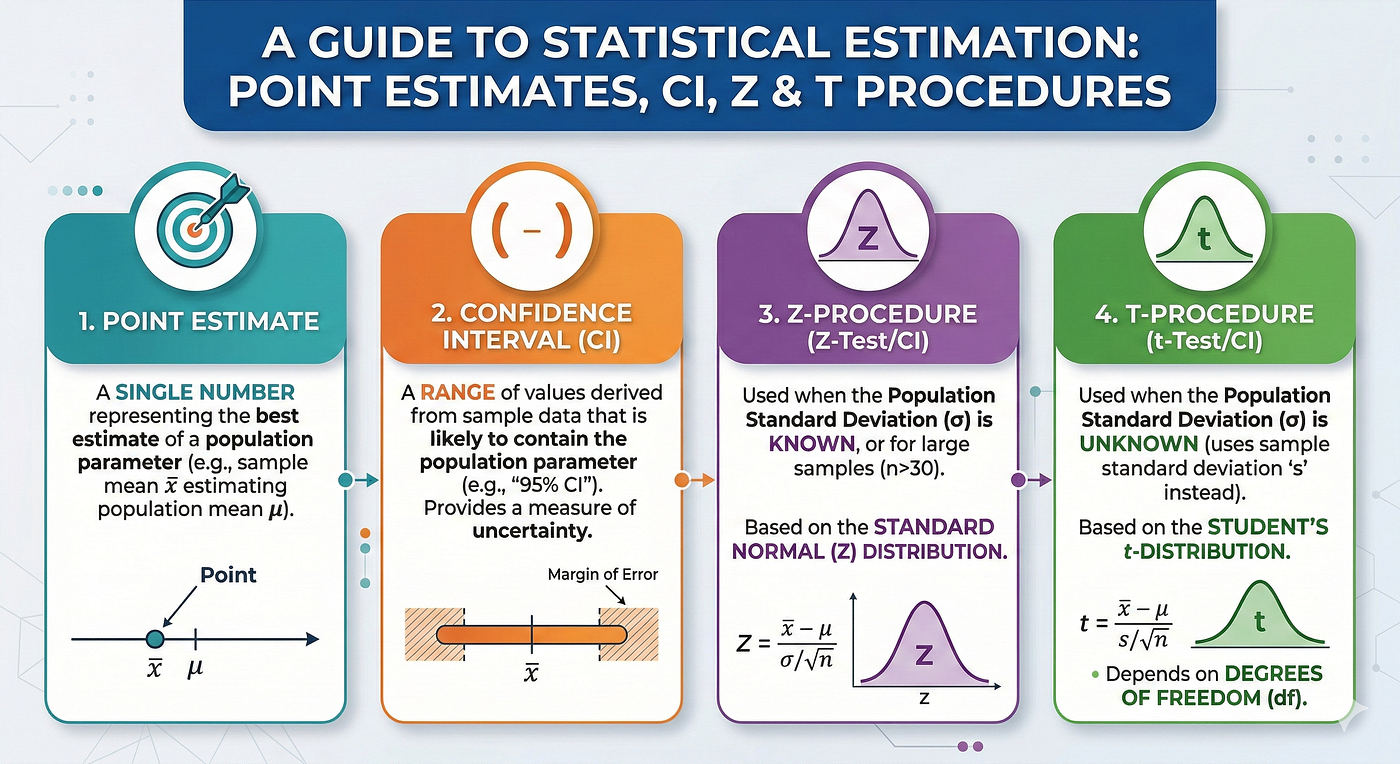
A point estimate is a single value, calculated from a sample, that serves as the best guess or approximation for an unknown population parameter, such as the mean or standard deviation. Point estimates are often used in statistics when we want to make inferences about a population based on a sample. Example: You want to know the average height of all adult women in a country (the population parameter). You measure 1,000 women and find their average height is 165 cm. That 165 cm is your point estimate. While a point estimate gives us a specific number, it doesn’t tell us how accurate that number actually is. That is where Confidence Intervals come in.

Confidence Interval (CI)

Confidence interval is a range of values within which we expect a particular population parameter (like a mean), is estimated to lie with a certain level of confidence. It’s a way to express the uncertainty and precision around a point estimate obtained from a sample of data. Confidence Level is expressed as a percentage like 95%, indicates how sure we are that the true value lies within the interval. Confidence Interval is created for Parameters and not statistics. Statistics help us get the confidence interval for a parameter.

Confidence Interval = Point Estimate +- Margin of Error

Examples of CI

To interpret the confidence interval values, consider the following points:

1. Confidence level: The confidence level (commonly set at 90%, 95%, or 99%) represents the probability that the confidence interval will contain the true population parameter if the sampling and estimation process were repeated multiple times. For example, a 95% confidence interval means that if you were to draw 100 different samples from the population and calculate the confidence interval for each, approximately 95 of those intervals would contain the true population parameter.

2. Interval range: The width of the confidence interval gives an indication of the precision of the estimate. A narrower confidence interval suggests a more precise estimate of the population parameter, while a wider interval indicates greater uncertainty. The width of the interval depends on the sample size, variability in the data, and the desired level of confidence.

3. Interpretation: To interpret the confidence interval values, you can say that you are “X% confident that the true population parameter lies within the range (lower limit, upper limit).” Keep in mind that this statement is about the interval, not the specific point estimate, and it refers to the confidence level you chose when constructing the interval.

Factors Affecting Margin of Error:

• Confidence Level (1-alpha): Increasing Confidence Level increases the Margin of Error.

• Sample Size: margin of error reduces to a certain point there after increasing sample size has not much benefit.

• Population Standard Deviation: On increasing Standard Deviation, Margin of Error linearly increases.

Ways to calculate CI:

**Z-procedure (σ is Known & n ≥ 30)):**

If you have standard deviation of population.

Assumptions: 1. Random sampling: The data must be collected using a random sampling method to ensure that the sample is representative of the population. This helps to minimize biases and ensures that the results can be generalized to the entire population.

2. Known population standard deviation: The population standard deviation (σ) must be known or accurately estimated. In practice, the population standard deviation is often unknown, and the sample standard deviation (s) is used as an estimate. However, if the sample size is large enough, the sample standard deviation can provide a reasonably accurate approximation.

3. Normal distribution or large sample size: The Z-procedure assumes that the underlying population is normally distributed. However, if the population distribution is not normal, the Central Limit Theorem can be applied when the sample size is large (usually, sample size n ≥ 30 is considered large enough). According to the Central Limit Theorem, the sampling distribution of the sample mean will approach a normal distribution as the sample size increases, regardless of the shape of the population distribution.

(1 — alpha)100% Confidence Interval for mean*

**T-procedure (σ not known & **n < 30):

If you don’t have standard deviation of population. Mostly used.

Assumptions: 1. Random sampling: The data must be collected using a random sampling method to ensure that the sample is representative of the population. This helps to minimize biases and ensures that the results can be generalized to the entire population.

2. Sample standard deviation: The population standard deviation (σ) is unknown, and the sample standard deviation (s) is used as an estimate. The t-distribution is specifically designed to account for the additional uncertainty introduced by using the sample standard deviation instead of the population standard deviation. If there are multiple samples taken, then avearge of all sample standard deviation is used.

3. Approximately normal distribution: The t-procedure assumes that the underlying population is approximately normally distributed, or the sample size is large enough for the Central Limit Theorem to apply. If the population distribution is heavily skewed or has extreme outliers, the t-procedure may not be accurate, and non-parametric methods should be considered. If the sample size is small (n < 30) and population is normally distributed.

4. Independent observations: The observations in the sample should be independent of each other. In other words, the value of one observation should not influence the value of another observation. This is particularly important when working with time series data or data with inherent dependencies.

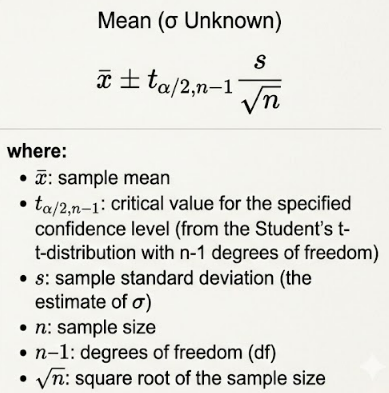
(1 — alpha)100% Confidence Interval for mean*

Student’s T Distribution:

Student’s t-distribution, or simply the t-distribution, is a probability distribution that arises when estimating the mean of a normally distributed population when the sample size is small and the population standard deviation is unknown. It was introduced by William Sealy Gosset, who published under the pseudonym “Student.” The t-distribution is similar to the normal distribution but has heavier tails. The shape of the t-distribution is determined by the degrees of freedom, which is closely related to the sample size. As the degrees of freedom increase (i.e., as the sample size increases), the t-distribution approaches the normal distribution.

degrees of freedom = sample size — 1

In hypothesis testing and confidence interval estimation, the t-distribution is used in place of the normal distribution when the sample size is small (usually less than 30) and the population standard deviation is unknown. The t-distribution accounts for the additional uncertainty that arises from estimating the population standard deviation using the sample standard deviation. To use the t-distribution in practice, you look up critical t-values from a t-distribution table, which provides values corresponding to specific degrees of freedom and confidence levels (e.g., 95% confidence). These critical t-values are then used to calculate confidence intervals or perform hypothesis tests.

NOTE: Given sample size and Confidence Level, t-value will be higher than z-value. For higher sample size, both t-value and z-value will be roughly equal.

Student’s T Distribution