Tensors, Euclidean Distance, Cross Product, Dot Product and Mean Centering

Tensor in Machine Learning

Tensor

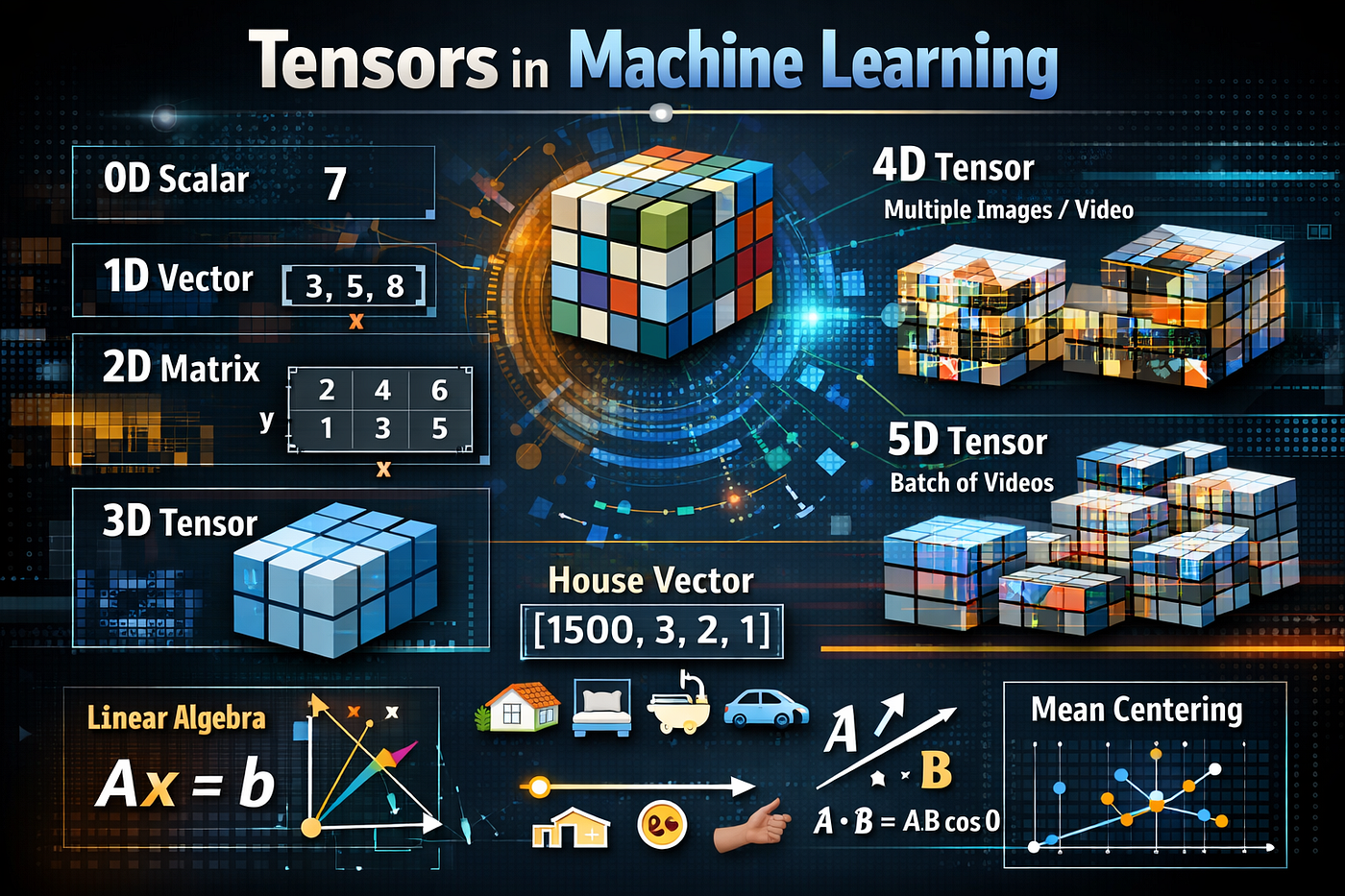
A tensor is a generalization of vectors and matrices and is easily understood as a multidimensional array. In the general case, an array of numbers arranged on a regular grid with a variable number of axes is known as a tensor. A vector is a one-dimensional or first-order tensor and a matrix is a two-dimensional or second-order tensor. Tensor notation is much like matrix notation with a capital letter representing a tensor and lowercase letters with subscript integers representing scalar values within the tensor. Many of the operations that can be performed with scalars, vectors, and matrices can be reformulated to be performed with tensors. As a tool, tensors and tensor algebra is widely used in the fields of physics and engineering. It is a term and set of techniques known in machine learning in the training and operation of deep learning models that can be described in terms of tensors. It is a type of datastructure or contains to store data mostly numbers. Examples : Scalar (0D), Vectors (1D), Matricies (2D), etc. Number of Dimentions is also called numbers of axis (Rank) we have in the tensor.

• 0D Tensor/Scalar: It has no dimentions. Examples: 2, 9 etc.
• 1D Tensor/Vector: It has one dimentions. Examples: [2, ] , [2, 9, 7, 8], etc.
• 2D Tensor/Matrix: It has two dimentions. Examples: [[2, 9, 7, 8],[2, 9, 7, 8]] etc.
• 3D Tensor: Example: One Image.
• 4D Tensor: Example: Multiple Images, one Video etc.
• 5D Tensor: Example: Multiple Videos.

NOTE: [2, 9, 7] is 1D Tensor or a Vector of 3D because it can only represented in 3 dimentions i.e. x, y and z axis only.

Linear Algebra

Linear algebra is a branch of mathematics that deals with the study of linear systems, which are sets of equations involving linear functions of variables. It is a foundational subject in mathematics and has applications in many areas, including computer science, engineering, physics, economics, and more.

It is used in ML:

• because good in generalizing concepts in higher dimentions
• Data Representation: we can represent tabular, text, image, video, etc data using it.
• work well with CPU and GPU for fast model development.

Vectors

It is a point in a coordinate system. An n-dimensional vector (n-vector) is an ordered list of n numbers, denoted as a tuple x = (x1, x2, x3,…,xn), representing a point or direction in n-dimensional Euclidean space. Each component x1 corresponds to a specific axis, generalizing 2D and 3D vectors to higher dimensions, commonly used for data representation, machine learning, and physics.

In machine learning, a vector is a numerical array (a list of numbers) used to represent data points, where each number corresponds to a specific feature or attribute of the object being described. This allows machines to process and perform mathematical operations (like calculating similarity) on various types of data, including text, images, and audio. Example: A specific house with 1500 sq. ft., 3 bedrooms, 2 bathrooms, and a garage would be represented by the vector: House Vector = [1500, 3, 2, 1] and it work as feaute input for model development and prediction. ML don’t work with Textual data, so we need to convert the text data into the vectors and train the model on the text.

Row and Column Vector:

x’s shape is n x 1, while a’s shape is 1 x n | (rows x columns)

Distance From Origin ||A|| or |A|: The distance between the origin and a point in n-dimensional space, we just need to sum up the squares of each coordinate and take the square root, as follows: For a vactor, v = (x1, x2,….., xn)

For n dimentions

Euclidean Distance

It is used in K-Nearest Neighbor (KNN), Classification Algorithm, etc.

• 2D Space: For two points(x1, y1) and (x2, y2), the distance d is

• n-Dimensional Space: For two points P = (p1, p2,…,pn) and (q1,q2,…,qn), the distance d is

Scalar Addition/Subtraction (Shifting): Use cases in ML mean centering etc.

• Scalar Addition: On adding n to a vactor, v = [v1, v2, v3, ….., vn], result = [v1 + n, v2 + n, v3 + n, ….., vn + n]
• Scalar Subtraction: On subtracting n to a vactor, v = [v1, v2, v3, ….., vn], result = [v1 — n, v2 — n, v3 — n, ….., vn — n]

Scalar Multiplication/Division (Scaling):

• Scalar Multiplication: On adding n to a vactor, v = [v1, v2, v3, ….., vn], result = [v1 n, v2 n, v3 n, ….., vn n]
• Scalar Division: On adding n to a vactor, v = [v1, v2, v3, ….., vn], result = [v1 / n, v2 / n, v3 / n, ….., vn / n]

Vector Addition/Subtraction

Process of adding two vectors by adding/subtracting their corresponding components.

Vector Addition | Vector Subtraction

Dot Product

It return scalar value. It is used to compute similarity between two vectors, calculate projection of A on B, Deep Learning and matrix multiplication.

If no of columns in a is equal to no of rows in b

Rules:

• Commutative:

• Distributive:

• Scalar Multiplication Rule:

• Dot Product with Itself:

Cross Product

It return vector value. An operation between two 3-dimensional vectors that produces another vector which is perpendicular to both original vectors.

Rules:

• Anti-Commutative: The order matters in cross product.

• Distributive:

• Scalar Multiplication Rule:

• Cross Product with Itself: The angle between them is 0°.

• Magnitude Formula:

• Parallel Vectors Rule: If vectors are parallel A×B = 0 because sin0 = 0
• Direction Rule (Right Hand Rule): The direction of A×B follows the Right-Hand Rule: ○ Point fingers in direction of A ○ Curl toward B ○ Thumb shows direction of A × B

Angle between 2 vectors

Cosine Similarity: The Cos of angle between two vectors A and B.

Angle between 2 vectors

If θ = 0 (cos θ = 1) then in same direction

If θ is 180 (cos θ = -1) means in opposite direction

If θ = 90 (cos θ = 0) then two vectors are perpendicular (orthogonal).

Unit Vector:

Projection of a vector:

Equation of line in n-D:

Equation of a Hyperplane: A hyperplane is a flat, (n-1)-dimensional subspace defined by the linear equation ω^T x + ωo = 0 that divides an n-dimensional ambient space into two distinct, separate half-spaces. As a fundamental concept in geometry and machine learning, it serves as a decision boundary (e.g., a line in 2D, a plane in 3D) used to separate data points into different classes. it is represented using pi, π.

2D

3D

N Dimentional

Standard Form where ω is normal vector, x is point vector and ωo is bias or offset

Vector Norms

Mean Centering

It is a useful pre-processing technique in various machine learning applications. It can improve the performance, convergence, and interpretability of the model. Some practical examples where mean centering is applied include:

Mean Centering

1. Principal Component Analysis (PCA): PCA is a dimensionality reduction technique that transforms the data into a new coordinate system by identifying the directions (principal components) with the highest variance. Before applying PCA, it is essential to mean center the data to ensure that the first principal component represents the direction with the highest variance in the dataset, rather than being influenced by the location of the data in the coordinate system.
2. Linear regression: In linear regression, mean centering can help improve the interpretability of the model coefficients by making them directly comparable. When the features are mean-centered, the intercept term represents the expected value of the dependent variable when all independent variables are at their mean values. Additionally, mean centering can help with multicollinearity issues, especially when there are interaction terms in the model.
3. Gradient-based optimization algorithms: Some machine learning algorithms, such as gradient descent, can converge faster when the input features are mean-centered. This is because mean centering can lead to better conditioning of the optimization problem, allowing the gradient descent algorithm to take larger, more consistent steps towards the optimal solution.
4. Clustering algorithms: Mean centering can help improve the performance of clustering algorithms like k-means by ensuring that the initial cluster centroids are not heavily influenced by the location of the data in the coordinate system. This can lead to faster convergence and better clustering results.
5. Regularization: In machine learning models that use regularization techniques, such as ridge regression or LASSO, mean centering can help ensure that the regularization term has a consistent effect across all features. By mean centering the features, the model is less likely to penalize the intercept term, which can lead to better generalization.

Matrix

A matrix is a rectangular array of numbers, symbols, or expressions arranged in rows and columns. The numbers, symbols, or expressions are called the elements of the matrix.

A matrix of order 3x3

Order of a matrix: Numbers of Rows x Numbers of Columns. Like 3x3 in the above figure.

Uses and Application Areas:

1. Linear Systems: Matrices can be used to represent and solve systems of linear equations. A system of linear equations can be written in matrix form as Ax = b, where A is the matrix of coefficients, x is the column vector of unknowns, and b is the column vector of constants. Methods such as Gaussian elimination, LU decomposition, and matrix inversion can be employed to find the solutions to the system.
2. Linear Transformations: Matrices are used to represent linear transformations between vector spaces. A matrix can define a linear transformation that maps vectors from one space to another while preserving the operations of vector addition and scalar multiplication. For example, rotation, scaling, and reflection transformations in geometry can be represented using matrices.
3. Eigenvalues and Eigenvectors: Matrices are used in the study of eigenvalues and eigenvectors, which are essential in various applications such as differential equations, stability analysis, and diagonalization of matrices. An eigenvalue-eigenvector pair (λ, v) of a square matrix A satisfies the equation Av = λv.
4. Graph Theory: In graph theory, matrices can be used to represent graphs through adjacency matrices, incidence matrices, and Laplacian matrices. These matrix representations provide a convenient way to analyze the properties of graphs and perform operations on them.
5. Markov Chains: Matrices are used in the study of Markov chains, which are stochastic processes that undergo transitions from one state to another according to certain probabilistic rules. Transition matrices describe the probabilities of transitioning between different states in a Markov chain and can be used to analyze the long-term behavior of the system.
6. Computer Graphics: Matrices are used extensively in computer graphics to represent transformations such as translation, rotation, scaling, and projection. These transformations are applied to 2D or 3D models to manipulate their position, orientation, and size in a virtual environment.
7. Control Theory: In control theory, matrices are used to represent and analyze linear systems, such as state-space models and transfer functions. The use of matrices in control theory allows for the design and analysis of control strategies for complex systems.
8. Optimization: In optimization problems, matrices can be used to represent constraints, objectives, and variables. Techniques such as linear programming, quadratic programming, and semidefinite programming rely on matrices and matrix operations to find optimal solutions.

Types of Matrices

• Row Matrix/Row Vector:

Row Matrix

• Column Matrix/Column Vector:

Column Matrix

• Square matrix(diagonal): In Square Matrix, diagonal elements are those elements for which i = j.

Square matrix

• Non-square Matrix:

Non-square Matrix

• Diagonal Matrix:

Diagonal Matrix

• Scalar Matrix: It has any constant value on the main diagonal.

Scalar Matrix of 1x1 and constant 1

Scalar Matrix of 3x3 and constant 3

• Identity Matrix: It always have 1s on the main diagonal.

Identity Matrix

• Zero Matrix/Null Matrix:

Zero Matrix

Matrix Equality

Two Matrices are equal if Order should be same and Aij = Bij

Order of A and B are 2x2 and every corresponding elements are equal

Scalar Operation

• Scalar Addition: If order of two matrix are same.

Scalar Addition

• Scalar Multiplication: Rules: k(A + B) = kA + kB and (k + l)A = kA + lA

Scalar Multiplication

• Negative of a Matrix:

Negative of a Matrix

Matrix Addition and Subtraction

• Matrix Addition:

Matrix Addition

• Matrix Subtraction: We first multiple B with -1 and add A and -1 x B using Matrix Addition.

Rules

• Order of Two Matrix A and B must be same.
• Commutative Law: A+B = B+A
• Associative Law: (A+B)+C = A+(B+C)
• Existence of additive identity: Let A = [aij] be an m × n matrix and O be an m × n zero matrix, then A + O = O + A = A. In other words, O is the additive identity for matrix addition.
• The existence of additive inverse: Let A = [aij] m × n be any matrix, then we have another matrix as — A = [– aij] m × n such that A + (– A) = (– A) + A= O. So — A is the additive inverse of A or negative of A.

Matrix Multiplication

Only Possible number of columns is equal to number of rows and the shape of output Matrix will be number of rows x number of columns.

NOTE: Commutative Law is not Valid i.e. A.B! = B.A

Rules:

• Associative Law: (AB)C = A(BC)
• Distributive Law: A(B+C) = AB+AC or (A+B) C = AC + BC
• Multiplicative Identity: For every square matrix A, there exist an identity matrix of same order such that IA = AI = A.

Transpose of a Matrix

Order changes from n x m to m x n.

A′ is Matrix Transpose of A

Rules:

• (A′)′ = A
• (kA)′ = kA′ (where k is any constant)
• (A + B)′ = A′ + B′
• (A B)′ = B′ A′

Symmetric Matrix

A square matrix A = [aij] is said to be symmetric if A′ = A, that is, [aij] = [aji] for all possible values of i and j.

Symmetric Matrix

Skew Symmetric

A square matrix A = [aij] is said to be skew symmetric matrix if A′ = — A, that is aji = — aij for all possible values of i and j. Now, if we put i = j, we have aii = — aii. Therefore 2aii = 0 or aii = 0 for all i’s. This means that all the diagonal elements of a skew symmetric matrix are zero.

Skew Symmetric

Rule:

• For any square matrix A with real number entries, A + A′ is a symmetric matrix and A — A′ is a skew symmetric matrix.
• Any square matrix can be expressed as the sum of a symmetric and a skew symmetric matrix.

Invertible Matrices

If A is a square matrix of order m, and if there exists another square matrix B of the same order m, such that AB = BA = I, then B is called the inverse matrix of A and it is denoted by A-¹. In that case A is said to be invertible. Only Square Matrix with Non-Zero Determinant (Non-Singular Matrix) can be inverted.

Invertible Matrices

Determinant

It is a scalar value computed from a square matrix (a matrix with the same number of rows and columns) that carries important information about the matrix. It has several uses in linear algebra, including determining the invertibility of a matrix, finding the solution to systems of linear equations, and calculating the volume scaling factor for linear transformations.

Why determinant is possible only for square matrix? The interpretation of the determinant as a scaling factor is only meaningful for square matrices because the input and output spaces must have the same dimension for this concept to be applicable but dimension of output changes for non-square matrix.

What does it mean to have a negative determinant?

Negative Determinant means the matrix has fliped the orientation.

2D example of -ve determinent

What happens when a matrix is singular?

If you are in 2D then output is in 1D. If you are in 3D then output is in 2D and so on.

• Determinant of a matrix of order 1x1:

• Determinant of a matrix of order 2x2:

Order of A is 2x2

• Determinant of a matrix of order 3 × 3:

Rules:

• det(A) = det(A’)

A matrix with Zero Determinant is called Singular Matrix.

• Determinent Visualization

|A| = 1 and |B| = wh

Here, A is unit Vector, |A| = 1 and B is unit Vector multiplied by B. So, |B| = wh

|A| = ration of (Area of the matrix)/(Area of the Identity Matrix of the same order) and determinent of Identity matrix is always 1.

• Determinent = 0

Transform 2D to 1D

Minor

Minor of an element aij of a determinant is the determinant obtained by deleting its ith row and jth column in which element aij lies. Minor of an element aij is denoted by Mij.

Determinant of a Matrix A

NOTE: Minor of an element of a determinant of order n(n ≥ 2) is a determinant of order n — 1.

Cofactor

Cofactor of an element aij , denoted by Aij is defined by Aij = (–1)i + j Mij , where Mij is minor of aij.

• Minor and Cofactor of a matrix of order 2 × 2:

• Minor and Cofactor of a matrix of order 3 × 3:

NOTE: Sum of the product of elements of any row(or col) with their corresponding cofactors is equal to Determinant.

Adjoint of a matrix

The adjugate of a matrix, also known as the classical adjoint, is a matrix formed by replacing each element in the original matrix with its corresponding cofactor and then taking the transpose of the resulting matrix. The adjugate of matrix A is denoted as adj(A). The adjoint of a square matrix A = [aij] n × n is defined as the transpose of the matrix [Aij] n × n , where Aij is the cofactor of the element aij . Adjoint of the matrix A is denoted by adj A.

Rule:

• A(adj A) = (adj A) A = A I , where I is the identity matrix of order n.
• If A and B are nonsingular matrices of the same order, then AB and BA are also nonsingular matrices of the same order.
• The determinant of the product of matrices is equal to product of their respective determinants, that is, AB = A B , where A and B are square matrices of the same order.
• A square matrix A is invertible if and only if A is nonsingular matrix

Inverse of Matrix

It acts as a “reciprocal” (reversing the transformation) for matrices, allowing the “undoing” of a matrix operation, provided the original matrix is square and its determinant is not zero.

An inverse matrix is a matrix that, when multiplied by the original matrix, results in the identity matrix. The inverse matrix is defined only for square matrices (matrices with the same number of rows and columns) and not all square matrices have an inverse.

A matrix is invertible (has an inverse) if and only if it is non-singular, meaning its determinant is non-zero. If the determinant of A is zero, A is called a singular matrix, and it does not have an inverse. Inverse matrices play a crucial role in linear algebra and have many applications, such as solving systems of linear equations, finding the solution to a matrix equation, and performing various matrix operations. There are several methods for finding the inverse of a matrix, including Gaussian elimination, the adjugate method, and LU decomposition.

Inverse of Matrix

Solving a system of linear equations using Matrix:

Basis Vector

A basis vector is one of a set of linearly independent vectors that span a complete vector space, acting as the fundamental building blocks or coordinate axes for that space. Any vector in the space can be uniquely represented as a linear combination of these basis vectors. Example: If you have a vector [-2, 1] then it’s scalar values can be represented using -2i +j where i and j are unit vector or basis vector and we add them to create a linear combination. The blue and orange vectors are the elements of the basis or unit vector; the green vector can be given in terms of the basis vectors.

2D Vector

Linear Transformations

It is a type of mathematical function, 𝑇(𝑣), that maps vectors from one vector space to another while preserving the operations of vector addition and scalar multiplication. It acts as a geometric transformation (rotation, scaling, or shearing) that keeps straight lines straight and the origin fixed. Any Matrix operation can be called as Linear Transformation. Transformation act as Function which transform the input vector on multiplying with a matrix.

Black will change to Red || Green will change to Purple

Black will change to Red

3D

Yellow changed to Pink

Matrix Multiplication as Composition of Transformation

It is defined as the composition of two linear transformations, where the transformation represented by matrix B is applied first, followed by the transformation represented by matrix A(A.B). The resulting matrix AB represents the combined effect of these consecutive transformations.

NOTE: B will be multipled first because we always multiple vector from right side.

**Example 1:**

Original

Applying A on Original

Applying B on result of A on Original

Example 2:

Blue is Original and Red is after first Transformation

Blue is Original and Red is after two Transformations

NOTE: The first Matrix is the Entire Coordinate Space on which the first transformation is applied.

Test of Commutative Law

A.B =! B.A

B.A vs A.B

Associativity

(AB)C = A(BC)

(AB)C means first apply (C then B), then A

A(BC) means applying C, (then B then A)

means both are same as order of applying is same.

Transformation for Non-Square Matrix?

Square matrices (n × n) represent linear transformations where the domain and codomain vector spaces have the same dimensions, i.e., T: V → V. In these cases, the transformation maps a vector space onto itself. Non-square matrices can also represent linear transformations between vector spaces with different dimensions.

Tall Matrix: rows are greater than columns.

Example: If input is order 3x2 then output will be a plan (2D) in 3D space and if input is order 4x2 then output will be a plan (2D) in 4D space.

Wide matrix: columns are greater than rows.

Example: If input is order 2x3 then output will be a 3D in 2D space and if input is order 2x4 then output will be a 4D in 2D space.

NOTE: Area don’t exist for Non-Square Matrix.

Why only square matrix has inverse?

An inverse is possible only for square matrices because it is related to the concept of a matrix being a bijective linear transformation, which implies both injectivity (one-to-one) and surjectivity (onto). A square matrix represents a linear transformation between vector spaces of the same dimension, where the domain and codomain are the same. When a square matrix is invertible, its linear transformation is bijective, meaning that it has a unique inverse transformation. Transformation of Non-Square matrix delete losses the information about the data thus reverse is not possible. Let’s consider why non-square matrices cannot have inverses:

1. If a matrix A has more rows than columns (m > n), i.e., a tall matrix, the linear transformation it represents is from a lower-dimensional space to a higher-dimensional space. In this case, the transformation is generally not surjective (onto), as there are output vectors in the higher-dimensional space that have no corresponding input vector. Consequently, there is no inverse transformation that can map every output vector back to an input vector.
2. If a matrix A has more columns than rows (m < n), i.e., a wide matrix, the linear transformation it represents is from a higher-dimensional space to a lower-dimensional space (dimension reduction). In this case, the transformation is generally not injective (one-to-one), as multiple input vectors can map to the same output vector. Consequently, there is no unique inverse transformation that can map each output vector back to a unique input vector.

Again, the inverse of a matrix is possible only for square matrices because these matrices represent linear transformations between vector spaces of the same dimension. Only in these cases can a matrix potentially satisfy the conditions of being a bijective transformation, i.e., both injective and surjective, which allows the existence of a unique inverse transformation. However, not all square matrices have inverses; only those that are non-singular (with a non-zero determinant) have an inverse.

Why inverse is possible for non-singular matrices only?

Singular matrix transform the matrix from higher dimention into lower dimention example from 2D to 1D (same as Non-Square Matrix). Thus, reverse is not possible for square matrix.

Hadamard product

The Hadamard product, also known as the element-wise product or Schur product, is a binary operation that takes two matrices of the same dimensions and produces a third matrix where each element is the product of the corresponding elements of the input matrices. Specifically, given two matrices A and B of the same size m × n, their Hadamard product C is also an m × n matrix, where each element is defined as:

C[i, j] = A[i, j] * B[i, j] for all i = 1, …, m and j = 1, …, n.