Thrustworthy Machine Learning: Gradient/Decomposition-based XAI: GradCAM

Grad-CAM (Gradient-weighted Class Activation Mapping) is a technique designed to produce ‘visual explanations’ for decisions made by a wide range of Convolutional Neural Network (CNN)-based models, thereby making them more transparent and explainable.

Its primary goal is to help users understand why a deep neural network predicts what it predicts. This interpretability is crucial for building trust in intelligent systems and for their meaningful integration into daily life.

To support trustworthy machine learning, Grad-CAM provides a range of benefits that enhance the reliability and fairness of deep learning systems. First and foremost, it improves transparency and interpretability by visually highlighting the regions in an image that contribute most to a model’s decision. This allows users to understand the reasoning behind predictions better, even when they don’t have technical expertise.

By making the model’s internal logic visible, Grad-CAM helps build appropriate levels of trust between users and AI systems. It also plays a valuable role in diagnosing errors by showing why a model may have made an incorrect prediction, revealing that even seemingly flawed outputs can have underlying logic.

Ultimately, by helping identify and correct such issues, Grad-CAM contributes to the development of models that generalize better to real-world data and behave in more ethically responsible ways.

We call Grad-CAM a gradient-based method because it uses the gradients of the class score with respect to the feature maps in the final convolutional layer. These gradients serve as a signal to weight the importance of each feature map, enabling the generation of class-discriminative heatmaps.

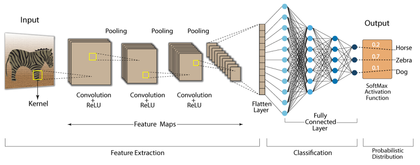
Now, we can visualize and explain each step of GradCAM by using the diagram below:

Section 1: Convolutional Layers (Feature Extraction)

The input image passes through multiple convolutional layers. These layers output feature maps (Aᵏ), where each feature map corresponds to a different filter or neuron.

Section 2: Grad-CAM (Gradient-weighted Class Activation Mapping)

Once the feature maps (Aᵏ) are generated by the convolutional layers, the following steps are applied to compute the class-discriminative saliency map using the Grad-CAM method

Step 1: Forward Pass & Class Selection

Perform a forward pass to obtain the raw output scores (logits) and select the target class c, usually the top predicted class.

Step 2: Backward Pass (Gradient Computation)

Backpropagate the class score yᶜ (before softmax) with respect to the feature maps Aᵏ.

This gives the sensitivity of each spatial location (i,j) in feature map Aᵏ for class c.

Step 3: Calculate Importance Weights (αᶜₖ)

Compute the average of the gradients over spatial dimensions:

Z: Total number of spatial locations in the feature map (i.e., Z=i×j)

Step 4: Combine Feature Maps and Apply ReLU, and Generate the Saliency Map

Multiply each feature map Aᵏ with its importance weight αᶜₖ, sum over k, and apply ReLU to focus only on features that positively influence:

This produces the final class-discriminative saliency map, highlighting image regions that positively contribute to class c.

Step 5: Visualise the results

Resize the resulting saliency map to match the original image size. Overlay it onto the original image to highlight the regions contributing to the selected class prediction.

Python Code for GradCAM

import torch
import torch.nn.functional as F
from torchvision import models, transforms
from PIL import Image
import numpy as np
import matplotlib.pyplot as plt
import cv2
#!!If you apply the code using Google Colab, write the code below
from google.colab import drive
drive.mount('/content/drive')

# ----------- Preprocessing and Model Setup -----------
device = torch.device("cuda" if torch.cuda.is_available() else "cpu")

# Load pre-trained model (e.g., ResNet50)
model = models.resnet50(pretrained=True).to(device)
model.eval()

# Choose the target layer (last conv layer in ResNet50)
target_layer = model.layer4[-1]

# Image preprocessing
preprocess = transforms.Compose([
    transforms.Resize((224, 224)),
    transforms.ToTensor(),
    transforms.Normalize(mean=[0.485, 0.456, 0.406],
                         std=[0.229, 0.224, 0.225])
])

def load_image(path):
    img = Image.open(path).convert('RGB')
    return preprocess(img).unsqueeze(0).to(device)
def load_original_image(path):
    img = Image.open(path).convert('RGB')
    img = img.resize((224, 224))
    return np.array(img)

# ----------- Grad-CAM Core Logic -----------

class GradCAM:
    def __init__(self, model, target_layer):
        self.model = model
        self.target_layer = target_layer

        self.gradients = None
        self.activations = None

        # Hook the forward and backward pass
        target_layer.register_forward_hook(self.save_activation)
        target_layer.register_backward_hook(self.save_gradient)

    def save_activation(self, module, input, output):
        self.activations = output.detach()

    def save_gradient(self, module, grad_input, grad_output):
        self.gradients = grad_output[0].detach()

    def __call__(self, input_tensor, class_idx=None):
        # Forward pass
        output = self.model(input_tensor)

        if class_idx is None:
            class_idx = output.argmax(dim=1).item()

        # ----------- Step 1: Compute Gradients of Class Score -----------
        score = output[0, class_idx]
        self.model.zero_grad()
        score.backward()

        # ----------- Step 2: Calculate Importance Weights (αᶜₖ) -----------
        grads = self.gradients  # [B, C, H, W]
        pooled_grads = torch.mean(grads, dim=[2, 3])  # Global average pooling

        # ----------- Step 3: Combine Feature Maps and Apply ReLU -----------
        activations = self.activations  # [B, C, H, W]
        for i in range(activations.shape[1]):
            activations[:, i, :, :] *= pooled_grads[:, i].unsqueeze(-1).unsqueeze(-1)

        heatmap = torch.sum(activations, dim=1).squeeze()
        heatmap = F.relu(heatmap)  # Apply ReLU to focus on positive contributions

        # Normalize and convert to NumPy
        heatmap = heatmap.cpu().numpy()
        heatmap = (heatmap - heatmap.min()) / (heatmap.max() - heatmap.min() + 1e-8)

        return heatmap, class_idx

def overlay_heatmap(heatmap, image_path, alpha=0.6):
    img = cv2.imread(image_path)
    img = cv2.resize(img, (224, 224))
    heatmap = cv2.resize(heatmap, (224, 224))
    heatmap_colored = cv2.applyColorMap(np.uint8(255 * heatmap), cv2.COLORMAP_JET)
    overlay = cv2.addWeighted(img, 1 - alpha, heatmap_colored, alpha, 0)
    return overlay

# ----------- Run on Example Image -----------

# Set your image path
image_path = "your image" # Write your patch of image here 

# Generate Grad-CAM heatmap and overlay
input_tensor = load_image(image_path)
gradcam = GradCAM(model, target_layer)
heatmap, class_id = gradcam(input_tensor)
overlay = overlay_heatmap(heatmap, image_path)

# Load original image for comparison
original_image = load_original_image(image_path)

# ----------- Plot: Side-by-Side Comparison -----------
plt.figure(figsize=(12, 5))

# Original
plt.subplot(1, 3, 1)
plt.imshow(original_image)
plt.title("Original Image")
plt.axis("off")

# Grad-CAM Overlay
plt.subplot(1, 3, 2)
plt.imshow(cv2.cvtColor(overlay, cv2.COLOR_BGR2RGB))
plt.title(f"Grad-CAM (Class {class_id})")
plt.axis("off")

plt.tight_layout()
plt.show()

In short, Grad-CAM is a method used to visualize which parts of an image a deep learning model focuses on when making a classification decision. It does this by generating a class-discriminative saliency map that highlights the image regions most relevant to the model’s prediction. The input is a regular image (e.g., a bird photo), and the output is a heatmap overlaid on the image, showing the areas that contributed most to the predicted class.

References:

https://arxiv.org/pdf/1610.02391

https://www.researchgate.net/profile/Aditya-Chattopadhyay/publication/320727679/figure/fig9/AS:631199986892800@1527501212032/An-overview-of-all-the-three-methods-CAM-Grad-CAM-GradCAM-with-their-respective.png

https://arxiv.org/pdf/1611.07450