Distribution-based clustering with the Gaussian Mixture Model

Originally published here! It might be easier to read this article over there due to all the subscripts (idk if Medium.com supports them).

Hello fellow machine learners,

Last week, we introduced the Multivariate Gaussian distribution and explored how its parameters are a natural extension of the univariate distribution.

This time, we will apply that theory to help us understand a new ML algorithm: the Gaussian Mixture Model (GMM). So be sure to read last week’s article before jumping into this one:

All set? Then it’s unpacking time 📦

GMM: soft clustering

Similar to K-Means and DBSCAN, the Gaussian Mixture Model is a clustering algorithm.

The GMM aims to create Gaussian clusters and assign each data point to a cluster probabilistically. Suppose that our data points are d-dimensional, and that we have n such points. We can represent the n points as x1, x2, … , xn and define a dxn matrix x = ( x1, x2, … , xn) whose i-th column is simply the coordinates of the i-th data point.

Suppose further that we aim to create K Gaussian clusters to group the data into. Each Gaussian cluster will be defined by its own Multivariate Gaussian distribution, i.e.

Recall from last week that each μ_i is a mean vector, and each Σ_i is a covariance matrix.

Now the question becomes: for each data point x_i, which of the K Gaussians does it most likely belong to?

The goal is to figure out the underlying statistical distribution of the data, which we assume to be the linear combination of the K multivariate Gaussian distributions:

Here, N( x | μ_j, Σ_j) represents the probability density function of the j-th Multivariate Gaussian, which tells us the probability that the data point x is drawn from this distribution:

The coefficient π_j in front of the j-th Gaussian in (P) is called the mixing coefficient. It’s a weighting that determines the contribution of N(x | μ_j, Σ_j) to the overall mixture. We require that the components of the vector π = (π_1, π_2, … , π_K) sum to 1:

This setup is quite different to the K-Means and DBSCAN algorithms that we have discussed previously. With those algorithms, a data point either belonged to a cluster, or it didn’t. There was no in-between. Such algorithms are referred to as hard clustering techniques.

With the GMM, however, the nature of π suggests that a data point can belong to multiple clusters at once, with larger π_j values indicating that the input data point is more likely to belong to cluster j. For this reason, the GMM is called a soft clustering technique. Soft clustering mechanism is especially useful for real-world contexts, in which it often isn’t easy to group data into entirely disjoint clusters.

Additionally, we learnt last week that the parameters of the Multivariate Gaussian can be tweaked to not only move the main ‘bump’, but also to manipulate the spread of the bump’s values. This gives us far more control over the size and shape of each cluster compared to, say, K-Means.

Regardless, it’s clear that we want to maximise the probability (P), because that makes our choices of Multivariate Gaussian parameters (i.e. our cluster choices) more meaningful for the dataset.

Maximum Likelihood Estimation (MLE)

Suppose that the data x_1, x_2, … , x_n was generated from realisations of the n independent random vectors X_1, X_2, … , X_n. The probability of observing this data, given our K Multivariate Gaussians, is given by

We want to maximise the probability of the above. This depends on the values of the statistical parameters in our data, which we can collectively define as

The Maximum Likelihood Estimate can be written as

where the likelihood function is given by

To maximise a function with respect to a set of variables, we would usually apply a calculus technique, e.g. computing partial derivatives, setting them equal to zero and potentially solving a set of simultaneous equations. But this gets very complicated with our function f. Is there a way to at least estimate the values of Θ?

For a fixed data point x_i, define a variable z_i that tells us which Gaussian cluster x_i belong to. To encode this, we specifiy that:

• The variable z_i takes a value in {1,…,K}. If xi belongs to cluster j, then we set z_i=j.
• The probability of z_i being equal to j is given by the j-th mixing coefficient:

(In stats language, we say that z_i follows a categorical distribution of parameters 1 and π.)

We do not actually observe the value of any such z_i, and so we refer to them as latent variables. Although not seen, they help with writing out the maths. Speaking of which, we can say that

In words, this means that x_i comes from cluster j if the value of the corresponding latent variable indicates it.

Expectation Maximisation (EM)

Here are some questions you may have at this point:

❓ How do we find the optimal parameters ( μ_j, Σ_j) for each Multivariate Gaussian?

❓ For a given data point x_i, what is the correct soft labelling? That is, what are the values of z_i and π?

It feels as though we cannot answer this pair of questions at the same time. We need to know the parameters of each Gaussian cluster so that we can assign soft labels corresponding to the ‘nearest’ clusters. This can be done empirically if we know the value of each z_i. But as mentioned before, the z_i are latent variables: we cannot observe them. So how do we find the values we need if we don’t know where to start with either set? Not to mention that we also need the values of the vector π!

To resolve these issues, we follow the Expectation-Maximisation algorithm, which provides a general framework for approximating parameters. As the name suggests, it comes with two main steps.

First is…

🎯 Expectation: we compute estimates for the values for the latent variables, for fixed Gaussian clusters. We define w_{i,j} to be the probability that z_i=j given the data point x_i and fixed Gaussian clusters. We have by Bayes’ Rule that

We already know the distributions of the expressions in the numerator: remember that x_i | z_i=j follows the j-th Multivariate Gaussian distribution while P(z_i=j) = π_j.

What about the denominator? By the law of total probability, we can condition over all the possible values of z_i. We don’t have to write this out explicitly, but hey, what the heck:

Notice that the denominator is precisely the pdf of the Gaussian Mixture Model.

Now it’s time for…

⌨️ Maximisation: we compute estimates for Θ = {π, μ1, …, μK, Σ1, .. , ΣK} by using the values in wi,j.

We can update the values of π by taking the average of the wi,j:

The new Gaussian means and covariance matrices can be updated using the below:

These formulas arise from the Maximum Likelihood Estimators of the Multivariate Gaussian distribution.

We iterate over this pair of steps until we converge on suitable values for all the unknowns. So we initialise Θ at random, use these values to estimate the latent variables, apply these to update the components of Θ, and continue until convergence.

Gaussian Mixture Model: visualisation

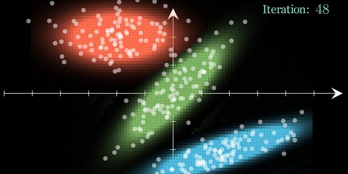
The following animation doesn’t quite do justice to the whole ‘soft clustering’ concept, but it’s still fun to look at how the Gaussian clusters move around over the training iterations:

Check out the original post on Substack; sadly the original video is too big to upload on Medium (booooo!)

Packing it all up

And that wraps up our discussion of the Gaussian Mixture Model! Here’s a quick roundup of what is a rather complex topic:

🔑 The Gaussian Mixture Model’s probability density function is a linear combination of Multivariate Gaussians. The mixing coefficients indicate the signficance of the corresponding Gaussian for the input data point.

🔑 Maximum Likelihood Estimation is a technique that can be used to find optimal parameters for a likelihood function. (We didn’t go into too much detail on MLEs though)

🔑 The Expectation-Maximisation framework can be used to find optimal mixing coefficients and Gaussian cluster parameters.

Training complete!

I hope you enjoyed reading as much as I enjoyed writing 😁

Do leave a comment if you’re unsure about anything, if you think I’ve made a mistake somewhere, or if you have a suggestion for what we should learn about next 😎

Until next Sunday,

Ameer

• My GitHub repo where you can find the code for the entire newsletter series: https://github.com/AmeerAliSaleem/machine-learning-algorithms-unpacked
• A blog that helped me put the code together for this week’s animation: https://www.oranlooney.com/post/ml-from-scratch-part-5-gmm/
• “The Whole and its Parts: Visualizing Gaussian Mixture Models”, by J. Giesen, P. Lucas, L. Pfeiffer, L. Schmalwasser, and K. Lawonn
• Maximum Likelihood Estimator for the Multivariate Gaussian: https://www.statlect.com/fundamentals-of-statistics/multivariate-normal-distribution-maximum-likelihood
• Stanford lecture notes on GMM and EM: https://web.stanford.edu/~lmackey/stats306b/doc/stats306b-spring14-lecture2_scribed.pdf

Originally published at https://ameersaleem.substack.com.