A Beginner’s Guide to Quantum Computing

Part 1: A beginner’s introduction to Quantum Computing using school-level maths

Quantum computing sounds intimidating. It doesn’t have to be.

This is the first article in Quantum Computing for You — A series for beginners who want to explore the next wave of technology without drowning in advanced maths. If you know basic school maths and are willing to read carefully, you’re in the right place.

I started learning quantum computing about two years ago. It was exciting and at times it felt like going down a rabbit hole. These articles are my attempt to explain the ideas simply, the way I wish someone had explained them to me.

Let’s start with the qubit

What is so special about a qubit which forced us to add qu in front of bit? The simple answer is that its behaviour is governed by principles from quantum physics. One of those principles is this: before we measure a qubit, we cannot treat it like a fixed 0 or 1. We can only describe the probabilities of getting 0 or 1.

When we measure a qubit, we always get one of two values: 0 or 1. Measurement forces the qubit into one definite outcome. After that, repeated measurements give the same answer. That is unlike a classical bit, which is always either 0 or 1 even before you look at it.

You might be wondering: so what? It still gives me a binary value. To appreciate what a qubit can do, we need to go a little deeper and be patient.

If you are seriously considering quantum computing as a frontier or career in the next few years, that patience will pay off.

The best explanation I have found for what this “in-between” behaviour feels like comes from Chris Bernhardt’s book, *Quantum Computing for Everyone*. Anyone serious about this path should read it as a starting point.

The Quantum Clock

This section adopts the concept from “Quantum Computing for Everyone” and explains the qubit.

Imagine a clock on the wall with only an hour hand. Your task is to find out the hour. The rules are:

1: Whenever you want to check the time, it tells you only if it’s 12 (up) or 6 (down)

2: Clock chooses to go to 12 (up) if the time is between 12:00 and 2:00 and 10:00 to 12:00.

3: Clock chooses to go to 6 (down) if the time is between 4:00 and 6:00 and 6:00 to 8:00.

4: At 3 and 9 it can choose 12 (up) or 6 (down) with equal chance.

5: You can check the time as many times as you like.

What can we learn from this?

1: If the true hour is 12, 1, 2, 10, or 11, the clock always shows 12 (up).

2: If the true hour is 4, 5, 6, 7, or 8, the clock always shows 6 (down).

With one check, you often learn whether the hour is in the upper half or lower half of the clock face.

Special Cases are 3:00 and 9:00.

If you check multiple times at one of those hours, you may sometimes get 12 and sometimes 6. That does not tell you whether it is exactly 3 or exactly 9; both behave the same way but it does tell that you are in the ambiguous zone, not at an hour like 1 or 7.

This clock is an analogy for a qubit.

The behaviour in condition 4 is what we call superposition:

1: Before measurement: the qubit has probabilities for up and down.

2: After measurement: you get one definite outcome.

Why does this lead to quantum algorithms?

Suppose you want to know the exact hour, not just upper half or lower half. You cannot get that from one check.

That question, how do we extract useful information from quantum systems?, is exactly where quantum algorithms come in. They are built as quantum circuits designed to steer the qubit (or many qubits) toward the answer you need.

We will come back to that in later articles. For now, let’s connect the clock to the maths.

Up and down in notation

A single-qubit state is written |ψ⟩ (read “ket psi”). Here, ψ is just a label for “the state we are talking about.” That state can be purely up, purely down, or a combination of both.

12 (up) → |0⟩ (read “ket zero”)

6 (down) → |1⟩ (read “ket one”)

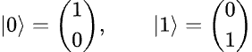
ket zero and ket one

At 3 or 9, the qubit isn’t simply |0⟩ or |1⟩ — In words: “half-weight toward up, half-weight toward down.”

That means:

50% chance of measuring 0 (up)

50% chance of measuring 1 (down)

Wrapping up

In this article, I tried to explain the qubit in simple terms — using the quantum clock rather than heavy physics.

In Part 2, we will go further into the basic maths, how notation works, what those numbers in a qubit state mean, and why they matter, and we will create the quantum NOT gate with basic mathematics.

Later in the series, we will go deeper into superposition, entanglement, and measurement — and then build toward gates, circuits, algorithms, and real hardware.

Coming in this series

Part 1 (this article): A Beginner’s Guide to Quantum Computing.

Part 2: The Magic of Maths in Quantum — kets, bras, projectors, operators and NOT gate.

Part 3: The Magic of Maths in Quantum — CNOT gate

Part 4: The Magic of Maths in Quantum — Superposition, Entanglement and Measurement

Part 5: The Magic of Maths in Quantum — Hadamard Gate

Later: Quantum circuits, algorithms, simulation, and real hardware

Most articles need only school-level maths and a willingness to read slowly.

Takeaways

A qubit is the quantum version of a bit; measurement always returns 0 or 1.

Unlike a classical bit, a qubit can be prepared so outcomes are not fixed before measurement.

The quantum clock shows this: most hours give a definite up or down; 3 and 9 give random up/down.

Further reading

[embed]CB info I am a professor emeritus of mathematics at Fairfield University. Originally from England, I came to the United States…www.chrisbernhardt.info

[embed]Quantum Computing for Everyone Quantum computing is a beautiful fusion of quantum physics and computer science, incorporating some of the most…mitpress.mit.edu