Predicting Protein Functions with GNNs
By Daniel Kumar, Anirban Chatterjee, Victor Samsonov for Stanford’s CS 224W course project
Predicting Protein Functions with GNNs
By Daniel Kumar, Anirban Chatterjee, Victor Samsonov for Stanford’s CS 224W course project

Background
Proteins are large molecules essential for numerous functions in our cells, tissues, organs, and overall body systems. Each protein is made up of a chain of 20 different amino acids, which can be represented as a sequence of length varying from 50 to >34,000 (averaging around 400–500) amino acids written in a 20-character alphabet (ACDEFGHILKMNPQRSTWVY). This unique sequence determines the protein’s structure and function. In many cases, even though we know a protein’s structure, we do not know its exact function in the cell.

Figure 1: Protein amino acid sequences of two polypeptide chains in the cow insulin hormone. (Image credit: OpenStax Biology, via Khan Academy)
To classify possible protein functions, the Gene Ontology (GO) Consortium provides a hierarchical classification system, using a dictionary of well-defined terms divided into three main categories (subontologies): molecular function, biological process, and cellular component. A protein’s function is then represented by one or more Gene Ontology (GO) terms, each term being associated with a given subontology. Researchers can query the GO database with a protein name to retrieve GO terms that have been associated with that protein using computational or experimental evidence.
The GO graph itself is a directed graph, where the sub-ontologies/GO terms (e.g. ‘GO:0048308 organelle inheritance’) are child nodes of the main categories and of one another:

Figure 2: Illustration of GO terms in relation to one another, and to the three overarching categories/subontologies (molecular function, biological process, and cellular component sub-ontologies).
The cardinality of the spaces concerned highlights the complexity of the protein function prediction problem: protein sequences can be as much as 34,000 amino acids long, and the function space comprises around 48,000 GO terms among all the three subontologies. A protein’s function may consist of one or more of these subontologies one or more GO terms, implying a multi-label classification problem.
Problem Statement
Types of protein function prediction and Gene Ontology structure
The general idea is homologous protein sequences should have some similarity of function. There are multiple different categories of techniques for protein function prediction including Homology based matching, Structure based methods, Genomic context methods and Network based methods.
In our work, we used the curated dataset provided by the CAFA6 Kaggle competition organizers, which contained 82,403 protein sequences and their corresponding GO terms.

Figure 3: Illustration of the protein function prediction problem. The blue nodes in the ontology represent the predicted function of this input protein. Note that the two leaf annotation nodes, one of which is “DNA translocase activity”, uniquely identify the entire ‘consistent subgraph’ of ancestor nodes. (Radivojac (2013), A (not so) Quick Introduction to Protein Function Prediction)
Our goal was to predict the correct set of GO terms associated with each protein, given the protein’s amino acid sequence. We hypothesized that two distinct signals would help us predict the correct sub-ontologies:
- Protein sequence similarity: Given the widely varying lengths of protein sequences (four orders of magnitude), this similarity task is nontrivial. We used a pre-trained protein language model to convert these sequences to standard embeddings which we then used as input feature vectors for a NN performing multi-label classification. Due to memory constraints associated with processing and storing dense vectors, a batching strategy was implemented. Additionally, some sequences were unable to fit in memory within our colab environment; as a result, sequence lengths above a threshold (8,922 characters) were split into subsequences which were processed individually and averaged to avoid loss of information.
- GO graph structure: As we show above, GO terms are interconnected through directed parent-child relationships. Accordingly, two different proteins, associated with closely connected but distinct GO terms, may ultimately have similar functions. To leverage this signal, we captured the connectivity of the GO graph by utilizing graph representation learning by applying message passing to capture the relationships between different GO terms via their shared network structure. As observed in later portions of our solution, two well-known Graph Neural Network architectures were used as essential components for the final model, these included GraphSAGE and GAT.
Given that a portion of the data we deal with can be represented as a graph, Graph Neural Networks are leveraged to effectively learn protein function prediction. If you are unfamiliar with this side of Machine Learning, we strongly recommend skimming through the CS 224W lecture slides.
We propose a powerful Multi-Tower architecture approach, which leverages the transductive graph scenario present in the CAFA 6 challenge allowing us to learn relevant node interactions within all three subontologies combined with the learned hidden state from a DNN which takes the protein embeddings as input.
Dataset and Preprocessing
For our prediction task, the architecture we chose was a multi-tower architecture, which combined the hidden state learned from protein sequences and the embeddings learned from the GO graph structure to create a unified representation (more details in the Methodology section below). Accordingly, in our data processing we preprocess the input features in several ways.

Figure 4: A sample of 0.05% of the GO graph in our data set. The nodes are GO terms, connected to one another by directed edges as in Figures 2 and 3 above. The nodes are colored according to which of the three main categories they fall within.
Protein sequence preprocessing
- To streamline the process of generating protein embeddings of different lengths in a consistent manner, we used the ESM-2 8M pre-trained Protein Language Model (PLM) to create one embedding (320 dimension) per protein sequence.
- Given the dataset size and available GPU/memory constraints, processing the entire training data sequence was not possible so we built a custom batching process and then stored the embeddings locally, so that we could reuse the generated embeddings without re-training or re-running inference each time. Additionally, to handle the largest sequences (>8,922 characters) effectively in memory, we chunked them up into smaller sequences and averaged the outputs of their subsequence embeddings.
- Finally, to alleviate memory constraints in our environment, dimensionality reduction was leveraged. We performed Principal Component Analysis (PCA) on the ESM output embeddings and reduced the embedding size to a dimension of 128. We chose this dimension because it allowed us to capture 95% of the variance.

Gene Ontology term and graph preprocessing
- We selected 600 distinct <protein, subontologies> pairs (by sampling the 200 highest frequency GO terms from each of the three ontology categories) in the training data to train our initial models. This reduced the GPU usage and let us iterate faster with different architectures.
- We represented each set of subontologies as a one-hot encoding vector, this can be observed in the code snippet below:

Figure 5a: Associating one-hot encodings for each EntryID by processing terms. Note that we added flexiblity to process all terms if needed.
- Additionally, since the .obo file which captures the graph metadata mixes all three subontology subgraphs, we performed processed our data to obtain each subotnology subgraph while keeping the edge directionality and injecting a virtual node to enhance message passing. The virtual node resulted in an enhanced F1-score for all of the experiments we performed. Based on initial iterations of our architecture, we realized that a lot of GO terms are disconnected from the rest of the subgraph, this sparsity is precisely why the introduction of a virtual node is beneficial.

Figure 5b: Associating one-hot encodings of GO subontology sets with protein IDs. This function also captures our introduction of a virtual node.
Challenges
- Our dataset is very sparse: although the GO graph is static, our protein dataset only contains 82,000 examples (compared to 40,000 subontology nodes), so most proteins have very few overlaps or trivial overlaps with one another in the subontology space.
- The data is highly imbalanced: as illustrated in Figure 6, a small subset of subontologies have multiple associations with proteins, while a long tail of subontologies have very few protein associations. This imbalance makes it difficult to identify multiple GO terms for a single protein using just protein data and the GO graph; more domain-specific representations underlying both the GO terms and protein structures will ultimately be needed in future work.
Below we present our EDA which showcases how quickly the number of terms decay as well as the long tail distribution. Also, we show a weak correlation of number of terms + protein sequence length, promoting the importance of preserving information as mentioned earlier in the protein sequence preprocessing (protein sequences above a specific threshold are chunked to obtain the embeddings and averaged over all chunks).

Figure 6: A selection of GO terms and the number of proteins with which they are associated. Note the wide range of associated protein counts; this selection is from the subset of 600 highest-cardinality GO terms so already excludes the long tail of GO terms with few or no protein associations. This pertains to the Molecular Function sub-ontology.

Figure 7: Long tail distribution

Figure 8: Weak correlation between Number of GO Terms and Sequence Length
Methodology
Once the data was processed, we performed experiments on a subset of GO terms (the 200 most common terms per subontology). A long tail distribution exists and the frequency for each term decreases rapidly leading to a setting where we have sparse vectors. Sampling the most common terms was done by Chervov et al. (2024) (arXiv:2412.04529), who trained their model on the ~5k most frequent terms. Less expressive models were used for less frequent terms to avoid overfitting. While we did not train specialized models for sparse terms (logistic regression for example) on the less frequent GO terms, we aimed to learn the sparser GO terms by using a loss function with weights assigned to prioritize less frequent terms.
In order to work around the data sparsity and imbalance issues described above, we experimented with multiple loss functions: binary cross-entropy, focal loss and a soft-F1 loss. The best performing loss was the soft-F1 custom loss. Training and validation sets were separated using a 95/5 split, specifically focusing on the 200 most common terms for each subontology. Our features underwent normalization and imputation where data was missing, while the predictions were made against the one-hot vectors of subontologies described above.
Relevant metadata was stored in a dictionary to easily map predicted one-hot values to their corresponding term.

Figure 9: Our weighted soft F1 loss calculation, implemented to help overcome our dataset imbalance and prioritize less frequently observed GO terms

Our experiments made use of three different model setups:
- 4-layer Deep Neural Network (protein embeddings as input)
- 4-layer DNN and GraphSAGE per subontology (protein embeddings as input for the DNN tower and 3 different GraphSAGE towers with a subontology graph as input).
- 4-layer DNN and GAT per subontology (protein embeddings as input for the DNN tower and 3 different GAT towers with a subontology graph as input).
It is important to note that when evaluating model performance, we use the following Github repo linked in the Kaggle competition which performs basic statistics including F-scores which is the main metric (customized by the CAFA competition organizers):
https://github.com/claradepaolis/CAFA-evaluator-PK
(expects ground_truth.tsv and to_score.tsv files)
Command to run: python src/cafaeval/main.py go-basic.obo predictions ground_truth_score.tsv
4-layer DNN Model
We consider our 4-layer Deep Neural Network to be a baseline to beat once we add graph-informed representations. While it does have expressive power, it is limited to the protein sequence embeddings processed; the GO graph context is not included in any way, considerably limiting some of its ability to generalize for more complex examples. These results are broadly reasonable, given that, modulo our GO term simplification, these results are on par with Kaggle’s current leading submission, which achieved a weighted f-score of 39.1%. Although we focus on only 600 GO terms, we do not use advanced techniques like concatenating protein embeddings from more than one strong model or train specialized models that each focuses on a unique sparse term. Below we plot the loss achieved during training for both training and validation while also including the average F1-score (some F1-scores are low, which is expected since the count for each term drops very quickly) and the best F1 scores for the top 3 terms.

Figure 10: Our 4-layer DNN Architecture, baseline
Multi-Tower Approach
Given a sensible baseline model, the remainder of this article will focus on the use of GNNs to enhance our predictive power with the help of our initial model, there will be 3 GNN towers and one DNN tower. We present a multi-tower approach which creates three separate GNNs for GraphSage, one per ontology category, and three separate GNNs for GAT. Our priority is to push the model to exploit the transductive setting of our data since the graphs provided will be static. This transductive setting promotes learning embeddings for all of the GO terms, which by leveraging a downstream attention mechanism allows protein logits to interact with the node graph embeddings for each subontology, helping proteins that contain those specific GO terms in the graph to obtain higher scores. This is an approach that appears to be less explored in CAFA competitions to date, per the literature we’ve seen so far.
Additionally, because of the sparsity of the graphs, we included self-loops in our initial experiments to allow for propagation of initial features. Unfortunately self-loops do not help much for isolated or disconnected subgraphs, these isolated sub-graphs/nodes would be largely ignored during training. Accordingly, we introduced a virtual node (see Figure 5), which allowed messages from all the disconnected nodes to be passed on, which resulted in the most highly performant approach so far. We believe a virtual node helps finding other relevant co-occurring terms as well as providing a stronger gradient signal for isolated sub-graphs. This is one of the major strengths of our implementation.
Our GNNs follow a similar structure where they are composed of 3 GCN layers, each including a dropout of 0.1 and a varying number of heads (1 head for GraphSAGE and 2 heads for the GAT implementation). When the number of layers was increased to 4 or 5 GCN layers, we observed diminishing returns and even worsened performance. We believe that some oversmoothing may be being introduced with higher numbers of layers.
Figure 11a: GraphSAGE forward and message function implementations.
Figure 11b: GAT forward and message function implementation.

Figure 11c: Multi-Tower class. Main idea is to include an attention head between graph nodes and protein scores
Since these GNNs are not explicitly used as a prediction head, a multi-tower setup is created where the logits from the DNN baseline model interact with the learned embeddings from all three subontology GNNs, via an attention mechanism. We then concatenate and process outputs through a final linear layer. Below we showcase a diagram for both GraphSAGE and GAT approaches:

Figure 12: Multi-Tower Architecture GraphSAGE

Figure 13: Multi-Tower Architecture GAT
Predicting Protein Function
Evaluation
We followed the evaluation methodology outlined by the CAFA6 Kaggle competition organizers to make sure we are able to benchmark the model accurately. Based on the competition guidelines, the maximum F1-measure based on the weighted precision and recall will be calculated on each of three test sets (for the three ontology categories MF, BP, and CC), and the final performance measure will be an arithmetic mean of the three maximum F-measures. The weights for the terms in each subontology are provided by the challenge organizers. The rationale for using weighted precision and recall is that GO is hierarchical and thus, the terms on top of the hierarchy are implied by their descendants. The weight for a term is determined by the logarithm of the frequency of occurrence of that term in a large pool of proteins. The root terms appear in every protein’s annotation and thus, their weights are 0. Terms deep in the ontology tend to appear less frequently, be harder to predict, and thus their weights are larger. The evaluation code is available on this GitHub repository.
Below we include the training plots for all of the relevant models, they are trained for 50 epochs, Adam optimizer, and a learning rate of 1E-4.
protein embeddings / NN predictor
DNN Training and Validation loss (soft F1)

Figure 13: Training and Validation Loss DNN. Label 52: F1 = 0.8888888888888888 Label 3: F1 = 0.6362957430918595 Label 183: F1 = 0.6153846153846154
Final f-score of 0.39
Multi-Tower GraphSAGE predictor
DNN Training and Validation loss (soft F1)

Figure 14: Training and Validation Loss GraphSAGE . 3 labels (best F1): Label 52: F1 = 0.6666666666666666 Label 3: F1 = 0.6362957430918595 Label 154: F1 = 0.61538461538461549

Final f-score of 0.48 (typo in screenshot, it is supposed to be GAT)
Multi-Tower GAT predictor
DNN Training and Validation loss (soft F1)

Figure 15: Training and Validation Loss GAT. 3 labels (best F1): Label 52: F1 = 1.0 Label 3: F1 = 0.6551433389544689 Label 154: F1 = 0.6274509803921569

Final f-scores of 0.46
We observe that these three models exhibited very different performances. The loss curve for the GAT and GraphSAGE enhancements had very noisy losses, which implies the possibility of further tuning the learning rate, allowing us to train longer. This noise likely comes due to the fact that when we initialize node embeddings to random values, they require considerable training to stabilize and are highly sensitive, we expect in future iterations to use a scheduler and warm up steps to improve training stability.
Top-3 F1 scores also are not a perfect metric to indicate stronger performance, as observed in the outcomes of the GAT approach. While it was able to achieve 100% for the top term (66% for GraphSAGE), it did not present a greater generalization capability compared to the GraphSAGE Multi-Tower when calculating the weighted F scores.
Protein function models are prone to overfitting, evaluating the use of simple models can boost the F1 score similarly to the approach proposed by Chervov because less expressive models have less chances to overfit when there is little data, as well as looking for better losses for our use case.
Overall, we conclude that models enhanced with graph structures of GO terms are able to capture the protein to term interactions much more effectively, this is in part thanks to the virtual node as well as the ability to observe relevant relationships between graph nodes and protein sequences by leveraging attention heads.
Future Work
- We used a standard PLM to create our embedding as it was trained on protein specific data. Enhancing PLM with a standard LLM finetuned using <Protein Sequence, GO terms> with RLHF can be an alternative path as well.
- PLM models generate dense embedding which might have limited expressiveness, other work has shown that using sparse autoencoders on top of dense embedding can help to create biologically meaningful features which might be more correlated to GO ontology structure.
- Finally, we have treated the problem as a homogenous graph problem whereas we can treat the GO graph as a relational graph with different types of relationships (is_a, regulates etc.) and nodes (C, F, P ontologies etc.). In that case the embedding might learn a richer characteristic from the interaction between different ontologies and relationships and be able to predict more accurately.
- We can also incorporate additional embeddings from ProtT5 as well as mining GO term semantic descriptions, an approach that proved to be very effective in CAFA5 top performing models.
- Explore other relevant secondary dataset to enhance the expressive power of our mode.
References:
[1] Chervov, A. (2024). ProtBoost: protein function prediction with Py-Boost and Graph Neural
Networks- CAFA5 top2 solution. arXiv:2412.04529
[2] Friedberg, I., Radivojac, P., et al. (2025). CAFA 6 Protein Function Prediction
https://kaggle.com/competitions/cafa-6-protein-function-prediction
[3] Gligorijevi´c, V., Renfrew, P. D., et al. (2021). Structure-based protein function prediction using
graph convolutional networks. Nature Communications, 12(1), 3168.
[4] Jiang, Y., Oron, T. R., et al. (2016). An expanded evaluation of protein function prediction
methods shows an improvement in accuracy. Genome Biology, 17(1), 184
[5] Radivojac, P., Clark, W., et al. (2013). A large-scale evaluation of computational protein function
prediction. Nature Methods 10 (3), 221–227.
[6] Zhao, C., Liu, T., & Wang, Z. (2022). PANDA2: Protein function prediction using graph neural
networks. NAR Genomics and Bioinformatics, 4(1).
메타데이터
- post_id
- 99fe008be27e
- slug
- predicting-protein-functions-with-gnns-99fe008be27e
- url
- https://medium.com/stanford-cs224w/predicting-protein-functions-with-gnns-99fe008be27e
- canonical_url
- https://medium.com/stanford-cs224w/predicting-protein-functions-with-gnns-99fe008be27e
- author_url
- https://medium.com/@victorsamsonov
- status
- ok
- fetched_at
- 2026-06-13 07:35:29