Data Modeling for Data Engineers: OLTP, OLAP, Inmon, and Kimball Explained

Understanding OLTP, OLAP, and the two roads your data can take after the transaction is recorded

Not a Medium member, you can read from here.

When I started learning data engineering, I kept running into the same cluster of terms: OLTP, OLAP, normalization, Inmon, Kimball, and star schema. I got confused by all of them and couldn’t see how they fit together.

They’re not separate topics.

They’re just different answers to the same question: how do we store data so it serves a specific purpose?

Instead of walking through definitions, I want to show you how they connect by following our customer, Mr. Data, from the moment he clicks checkout to the moment a data analyst runs a trend report about him.

By the end, you’ll see exactly where each term lives in that journey and why it exists.

OLTP to OLAP (Kimball and Inmon)

Stop 1: Mr. Data Places an Order — Meet OLTP

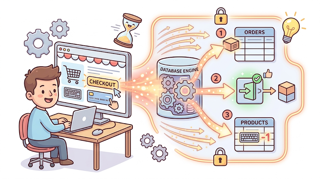
Mr. Data is browsing an online store. He finds a keyboard, adds it to his cart, enters his credit card number, and clicks checkout.

The moment he does, three things happen behind the screen:

• His order needs to be recorded correctly
• His payment needs to go through.
• The inventory count needs to drop by one.

It should not have delays, no half-written records, and no duplicates.

This is the job of an OLTP system — Online Transaction Processing.

The database sitting behind that checkout button is OLTP. It can be PostgreSQL, MySQL, or Oracle. These are built for one thing: handling a high volume of short, precise read-and-write operations correctly and fast.

When Mr. Data’s payment is processed, the inventory count has to drop at the same time. If the system crashes between those two operations, we can’t have the situation where his money is gone, but the keyboard is still showing as in stock.

OLTP databases enforce this through ACID properties:

• Atomicity — either the whole transaction happens, or none of it does
• Consistency — the database always moves from one valid state to another
• Isolation — two transactions happening at the same time don’t corrupt each other
• Durability — once committed, the data survives a crash

To make ACID work, OLTP databases use normalization — splitting data into many small, focused tables with no redundancy.

• Mr. Data’s name and address live in a customers table.
• His order lives in an orders table.
• The keyboard lives in a products table.
• They're all linked by IDs. Nothing is duplicated.

Normalization keeps writes clean: when a new order comes in, the database inserts one small, targeted record without touching anything that already exists. Also, if Mr. Data moves to a new address, we update it in one place only, rather than across thousands of historical order rows.

Here’s what Mr. Data’s order looks like in a normalized OLTP schema:

Customers              Orders                Order_Items
-----------            -----------           ----------------------
customer_id (PK)  ←── customer_id (FK)      order_item_id (PK)
first_name             order_id (PK)    ←── order_id (FK)
last_name              order_date            product_id (FK) ──→ Products
email                  status                quantity               -----------
address_id (FK)        payment_id (FK)       unit_price             product_id (PK)
    ↓                                                               product_name
Addresses          Payments                                         category_id (FK)
-----------        -----------                                      price
address_id (PK)    payment_id (PK)
street             amount
city               method
country            status

many tables, many foreign keys, minimal duplication.

Mr. Data’s order is now safely stored. The checkout worked, the payment cleared, and the inventory dropped. OLTP did its job.

However, after that data is captured, someone has to decide what to do with it next — and that decision is where the road splits.

Transactional Database

The Fork in the Road: Two Ways to Build a Warehouse

Three months pass. Mr. Data has placed more orders, as well as other customers. The business owner now wants to ask

• Which product categories drove the most revenue last quarter from millions of transactions?
• Which regions have the highest return rates?
• Which customers bought once and disappeared?

We will have a performance conflict if we answer them directly with OLTP, since the queries involve many joins due to the normalization.

-- Revenue by product category for Q3 2024
-- Requires joining 5 tables just to get to the numbers
SELECT
    p.category_id,
    SUM(oi.quantity * oi.unit_price) AS total_revenue
FROM order_items oi
JOIN orders o      ON oi.order_id    = o.order_id
JOIN customers c   ON o.customer_id  = c.customer_id
JOIN products p    ON oi.product_id  = p.product_id
JOIN payments pay  ON o.payment_id   = pay.payment_id
WHERE o.order_date BETWEEN '2024-07-01' AND '2024-09-30'
  AND pay.status = 'completed'
GROUP BY p.category_id;

This is why we need a data warehouse built for OLAP — Online Analytical Processing.

Snowflake, BigQuery, Redshift, DuckDB. These are optimized for reading large volumes of historical data fast, not for handling thousands of tiny writes per second.

Moving Mr. Data’s data into a warehouse solves the performance problem. But it doesn’t answer a harder question:

How should that data be structured inside the warehouse?

This is where two different philosophies for data warehouses come in: Bill Inmon and Ralph Kimball.

Both roads lead to a warehouse that can answer analytical questions. They just take opposite approaches to get there. Time to pick our route.

Road A: Inmon — Build the Enterprise Core First

Bill Inmon’s concern wasn’t the query. It was the data itself.

Mr. Data doesn’t exist in just one system

• His order lives in the e-commerce database
• His customer service history lives in a CRM
• His payment reconciliation lives in a finance platform
• His shipping events live in a logistics tool.

Each of those systems has a different ID for him, different field names, and a different definition of what a “customer” even means. Before any analyst runs a report, Inmon says, we have to resolve that mess.

His suggestion is to build a single, normalized enterprise data warehouse that integrates all source systems first — still in 3NF, same structural logic as OLTP — and treat that as the only one authoritative version of Mr. Data for the whole company.

Next, we create data marts using that clean core as the foundation. These are smaller analytical views designed for specific teams. For example, the e-commerce team gets a mart shaped for their specific needs, and finance gets another. We make sure Mr. Data remains one consistent record, so he stays the same in every report the company runs.

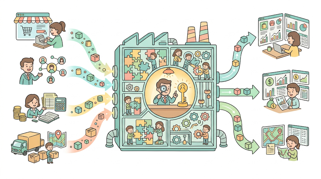
Center Datawarehouse with different data marts

This is Inmon’s top-down approach: the enterprise warehouse comes first, data marts come later.

Here’s what Inmon’s structure looks like in practice:

Source Systems
──────────────
E-commerce DB  ──┐
CRM            ──┼──→  Enterprise Data Warehouse  ──→  E-commerce Data Mart
Finance DB     ──┤      (Normalized, 3NF)          ──→  Finance Data Mart
Logistics      ──┘      Single source of truth     ──→  Logistics Data Mart
                         Mr. Data exists once

Next, let’s see another option Kimball provided to us.

Road B: Kimball — Flatten It, Ship It, Iterate

Ralph Kimball looked at the same problem and started from the other end: what do analysts actually ask?

He noticed that every analytical question has the same shape: How much of X, by Y, over time Z?

• Revenue by product category by quarter.
• Returns by region by month.
• Orders by customer segment by year.

The “how much” is always a number being aggregated. The ‘by’ clauses are your filters and groupings.

Therefore, Kimball thought that we could build the schema around that shape, so that analysts don’t need to reconstruct it through multiple joins.

• The “how much” becomes a fact table — one row per order line item, holding Mr. Data’s quantities, prices, and totals.
• The “by” dimensions — product, customer, date — become dimension tables surrounding it.

The technique that makes this possible is denormalization — the opposite of the OLTP and Inmon approach.

For example, we have address information and customer information, such as in two different tables in the transactional database. If we want to pull out Mr. Data’s name and where he lives. We need to join the address and customer, but now we can put them together into a table called dim_customer.

Here’s Mr. Data’s order data reshaped:

                           dim_customer
                          ----------------------
                          customer_key (PK) ─────→     
                          customer_name         |       
                          email                 |
                          street                |
                          city                  |
                          region                |
                          country               |
                                                |
                                                |

dim_date               fact_orders              |   dim_product
------------           -------------------------|    ----------------
date_key (PK)  ←────    date_key (FK)           |    product_name
full_date               customer_key (FK)─────→ |    category
day_of_week             product_key (FK)   ─────→    product_key (PK)    
month                   order_id (PK)                brand
quarter                 quantity                     unit_cost
year                    unit_price
                        total_revenue
                        order_status

When we put the fact table in the center and the dimensions around it, we get a star schema. Mr. Data’s order still exists, but now it’s been flattened and reshaped so an analyst can reach it in two joins instead of five.

-- Revenue by product category for 2024
-- Two joins. That's it.
SELECT
    p.category,
    d.quarter,
    SUM(f.total_revenue) AS revenue
FROM fact_orders f
JOIN dim_product  p ON f.product_key = p.product_key
JOIN dim_date     d ON f.date_key    = d.date_key
WHERE d.year = 2024
GROUP BY p.category, d.quarter
ORDER BY revenue DESC;

This is Kimball’s bottom-up approach: the data mart comes first, one business process at a time, and the warehouse grows around it.

Photo by Vitaly Gariev on Unsplash

Where Mr. Data Ends Up

The image below shows the journey Mr. Data went through from OLTP to OLAP.

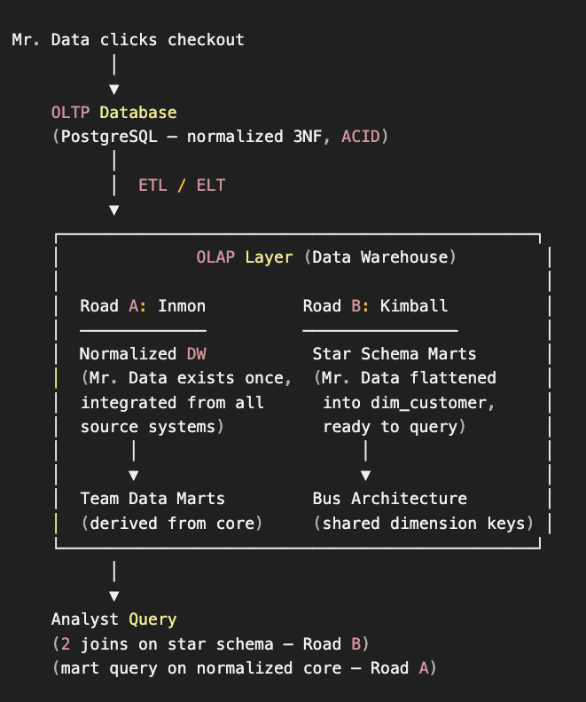
Mr Data Journey

Which Road Should You Take?

This is the question you may ask. Here are some directions we can think about before building a data warehouse.

• If you have multiple systems with conflicting definitions, like Mr. Data's information scattered everywhere, and need a single authoritative record before reporting, take Inmon.
• If you want to deliver fast, query-ready data and immediate value to your analysts, like putting all Mr. Data’s orders made in a year into a report, take Kimball’s star schema.

Sometimes, we may use both. In most modern stacks, dbt projects typically have a staging layer that preserves the normalized source structure — Inmon’s thinking — and a mart layer built on top with star schemas — Kimball’s output.

The Databricks medallion architecture (bronze, silver, gold) follows the same pattern. The gold layer is almost always a star schema.

Wrapping Up

There are lots of terminologies today, and I hope you got excited after reading this. Here is the quick summary of all of the terms we mentioned.

• OLTP and OLAP are workload types: OLTP protects the write, OLAP serves the read.
• Normalization is what makes OLTP fast and correct; denormalization is what makes the warehouse fast to query.
• Inmon says keep Mr. Data normalized in a single enterprise core and build team-specific marts from it. Kimball says flatten Mr. Data into a star schema from the start and integrate the marts through shared keys. Both of them are data warehouse concepts.

If you like this article and want to show some love:

• Clap 50 times — each one helps more than you think! 👏
• **Follow me**, so you won’t miss it when a new article is published
• You can buy m**e a Coffee** to support me further.
• Let’s connect with me at **LinkedIn or lhungen@gmail.com to chat more about data!**