Atari-Era DQN Tricks That Still Power Modern LLM Alignment

A practical walkthrough of how DeepMind’s Atari-era Deep Q-Networks work, and how their core ideas quietly reappear inside modern RLHF and RLVR pipelines for aligning large language models.

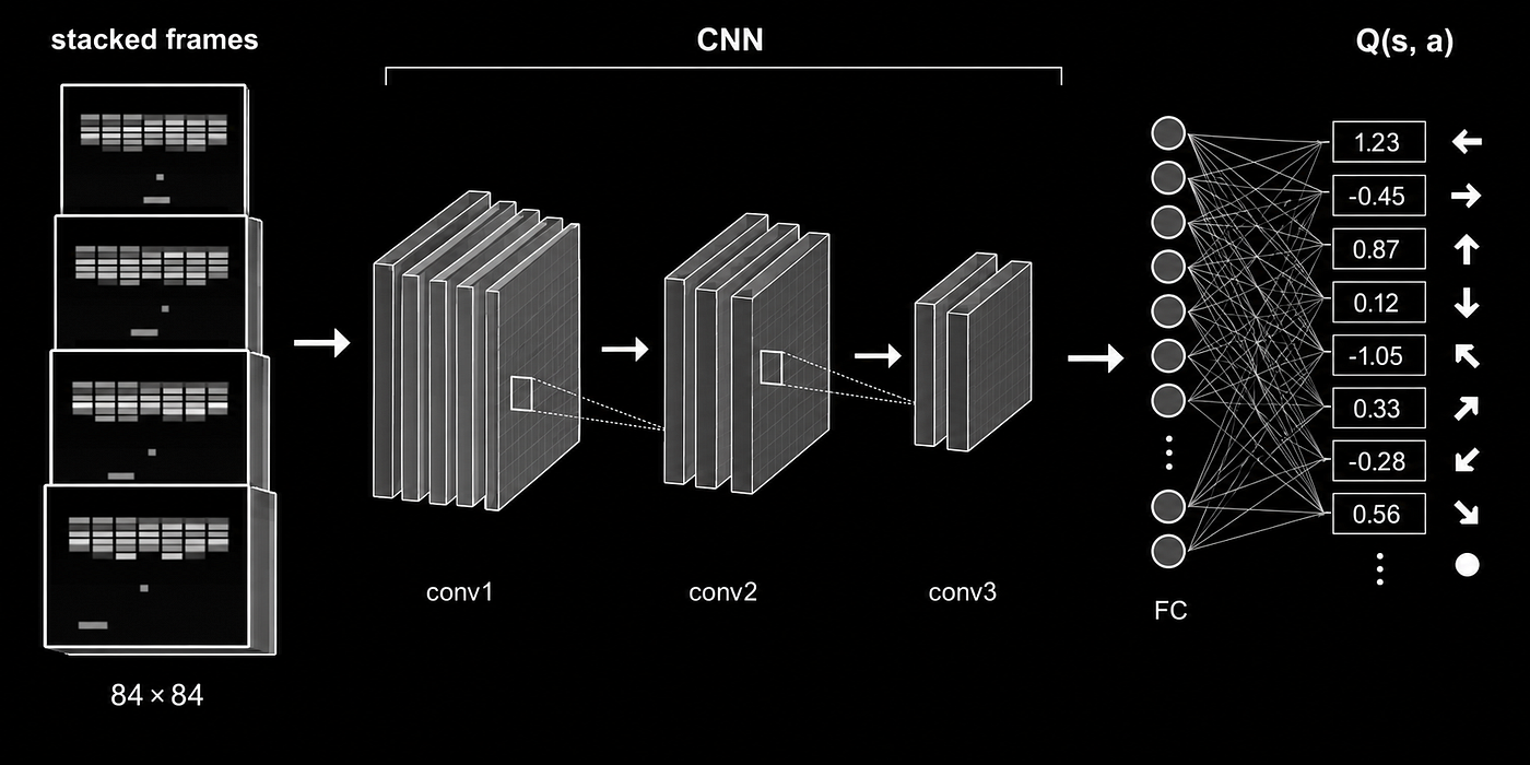
Classic Atari DQN: stacked frames in, a Q-value for every action out.

When people talk about “reinforcement learning from human feedback” (RLHF) and “reinforcement learning from AI feedback” (RLAF/RLVR), they rarely mention Atari 2600 games. Yet the same core idea that powered DeepMind’s Deep Q-Networks (DQNs) on Breakout and Space Invaders is still quietly sitting under many modern alignment pipelines for large language models (LLMs).

In this article, we will walk from classic Deep Q-learning on Atari, through the stabilizing tricks that made it work, and into the world of RLHF/RLVR for LLMs. Along the way, we will keep a practical engineer’s perspective and end with a minimal PyTorch-like DQN training loop you can actually recognize and adapt.

Why DQN Mattered in the First Place

Reinforcement learning (RL) frames decision-making as an agent interacting with an environment: it observes a state ss, takes an action aa, receives a reward r, and transitions to a new state s′. The goal is to learn a poa policy π(a∣s) that maximizes the expected sum of discounted rewards over time.

Value-based RL methods like Q-learning focus on the action-value function Q(s,a), defined as the expected return starting from state s, taking action aa, and following the optimal policy afterward. In tabular Q-learning, you update a table:

That works fine for tiny discrete problems grid worlds, toy MDPs but totally collapses when your “state” is a 210×160×3 Atari frame. You either need to handcraft features or learn to approximate Q(s,a) with a function approximator like a neural network.

Earlier attempts to combine Q-learning with neural networks were notoriously unstable. The core trick of DQN was to make this combination actually work on high-dimensional visual input by adding just enough stability mechanisms: convolutional networks, experience replay, and target networks.

The Deep Q-Network Recipe

At a high level, a DQN replaces the Q-table with a deep network Q(s,a;θ) that maps a state (stacked frames) to Q-values for all actions. It also maintains a separate target network Q(s,a;θ^-), which is a slowly updated copy of the online network.

The training loop looks like this:

• Interact with the environment using an ϵ-greedy policy over Q(s,a;θ).
• Store transitions (st​,at​,rt​,st+1​,dt​) in a replay buffer.
• Sample random minibatches from the replay buffer.
• Compute targets using the target network:
• If the episode ended: y = r.
• Otherwise: y = r + γ maxa′​ Q(st+1​, a′;θ^-).
• Minimize the mean squared TD error (y − Q(st​,at ;θ))².
• Periodically copy θ into θ^-.

DQN learns by replaying past transitions and updating a slowly copied target network.

Two stabilizing mechanisms are key:

• Experience replay breaks the temporal correlation of online trajectories and makes the training distribution more i.i.d.-like.
• Target networks prevent the “moving target” problem where you chase your own changing predictions.

The Atari Architecture

On Atari, the DQN architecture is a fairly standard convolutional stack:

• Input: stack of four 84×84 grayscale frames.
• Conv1: 32 filters, 8×8 kernel, stride 4, ReLU.
• Conv2: 64 filters, 4×4 kernel, stride 2, ReLU.
• Conv3: 64 filters, 3×3 kernel, stride 1, ReLU.
• FC1: 512 units, ReLU.
• Output: ∣A∣ linear units, one per action.

The key idea is that the network learns its own visual features directly from raw pixels, without hand-crafted representations. That “pixels to actions” story is exactly what captivated the RL community and set the tone for later deep RL work.

Training Details That Actually Matter

The original DQN paper and follow-ups highlight several “engineering details” that turned out to be non-negotiable:

• Frame skipping and action repeat to reduce temporal redundancy.
• Reward clipping to [−1,1] for stable gradients.
• Large replay buffers ( 10⁵–10⁶ transitions).
• Annealed ϵ-greedy exploration over millions of frames.
• Slowly updated target network (every tens of thousands of steps).

These may look like minor knobs, but in practice they are the difference between “paper-ready result” and “saturated NaNs and exploding Q-values”.

DQN as a Conceptual Template

Why dwell on DQN when we now have PPO, A3C, SAC, and a zoo of actor-critic algorithms?

Because DQN crystallized a core pattern that remains relevant:

• Learn a parametric value (or policy) function from high-dimensional input.
• Stabilize the bootstrapping process using some form of target network.
• Break correlation in the training data (replay, multi-environment rollouts, or off-policy data).
• Use simple reward signals to drive rich emergent behavior.

This basic template later informed:

• Off-policy algorithms for continuous control.
• Deep RL for resource management, traffic control, and edge computing.
• Hybrid planning and value-learning systems in model-based RL.

Even in domains where the exact algorithm is no longer “DQN”, the conceptual core value estimation plus stabilizing tricks remains.

From Atari Rewards to Reward Models

The real conceptual bridge from DQN to RLHF lies in how we think about reward.

In Atari, reward is simple: game score or some shaped variant of it. The environment provides a scalar signal, and we’re done. But for tasks like “be helpful, honest, and harmless” as a language model, there is no natural environment reward. We have to build it.

Modern work on reward models in deep RL explicitly generalizes that scalar reward into a learned function of state-action (or trajectory) pairs. You can think of this as upgrading from:

• Hard-coded r(s,a) from the environment, to
• A learned reward model Rϕ​(x) that predicts the quality of a model output x based on preferences, labels, or other signals.

In some sense, DQN taught us that you can learn a value function from noisy, bootstrapped targets and still get meaningful behavior if you stabilize the training loop. RLHF and RLVR extend this idea: you can learn a reward model from noisy preference data and still train a policy that behaves well, as long as you manage the instabilities in that larger loop.

RLHF: Turning Human Judgments into a Reward Signal

RLHF (Reinforcement Learning from Human Feedback) typically runs in three main phases:

• Supervised fine-tuning: Train a base policy on human-written data.
• Reward modeling: Train a reward model on human preferences over pairs of model outputs (e.g., “A or B: which is better?”).
• Policy optimization: Use reinforcement learning (often PPO-like policy gradients) to fine-tune the policy to maximize the reward model’s score.

RLHF adds a reward model and a PPO-style loop on top of a supervised-tuned LLM.

The last phase is structurally analogous to classic RL: the agent interacts with an environment (now a prompt-response loop), and receives a scalar “reward” from the learned model. The difference is:

• The environment dynamics are basically the model’s own outputs plus the prompt distribution.
• The reward is not external; it is a learned, possibly mis-specified, model.

Despite this, the same fundamental stability issues appear:

• Non-stationary reward and value targets as both policy and reward model evolve.
• Correlated trajectories and distributional shift.
• Over-optimization issues (reward hacking) when the policy exploits weaknesses in the reward model.

The DQN era already taught us that naive bootstrapping on non-stationary targets leads to divergence, and that careful engineering is required. RLHF frameworks reuse that lesson in a different regime.

RLVR and RL from AI Feedback

RLVR (Reinforcement Learning from Verifiable Rewards) and related approaches like RL from AI feedback partially automate the feedback loop by using auxiliary models or verifiable tasks instead of direct human preferences.

Examples include:

• Using automated test suites, constraints, or interpretable checks as reward signals.
• Using a “judge” model to compare outputs and provide preferences or scores.
• Using structured reward decomposition (e.g., separate correctness, style, and safety components).

RLVR replaces human scores with verifiable signals like tests or exact-match checks.

Again, this is conceptually close to RL with shaped rewards: we assemble a scalar reward from multiple signals and let the learning algorithm optimize it, with all the same dangers of misalignment and reward hacking.

From a DQN perspective, you can think of RLVR as “Atari, but the reward function is a program we wrote rather than a game’s built-in score”. The core RL machinery is similar; the complexity moved from the neural architecture into the reward and evaluation pipeline.

A Minimal DQN-Style Training Loop

To make this discussion concrete, here is a compact pseudo/PyTorch-style DQN training loop that captures the essence in roughly 20 lines. The point is not production-ready code but a mental model of how the moving parts fit together.

# Q-network and target network
q_net     = QNetwork().to(device)
target    = QNetwork().to(device)
target.load_state_dict(q_net.state_dict())
optimizer = torch.optim.Adam(q_net.parameters(), lr=1e-3)

replay = ReplayBuffer(capacity=100_000)
epsilon, gamma = 1.0, 0.99

state, _ = env.reset()
for step in range(1, max_steps + 1):
    # epsilon-greedy action selection
    if np.random.rand() < epsilon:
        action = env.action_space.sample()
    else:
        with torch.no_grad():
            q_values = q_net(torch.from_numpy(state).to(device))
            action   = q_values.argmax().item()

    next_state, reward, done, _, _ = env.step(action)
    replay.push(state, action, reward, next_state, done)
    state = next_state if not done else env.reset()[0]

    # decay exploration
    epsilon = max(0.1, epsilon - 1e-5)

    # train once buffer has enough samples
    if len(replay) < batch_size:
        continue

    states, actions, rewards, next_states, dones = replay.sample(batch_size)

    q_values = q_net(states).gather(1, actions.unsqueeze(1)).squeeze(1)
    with torch.no_grad():
        next_q = target(next_states).max(1).values
        targets = rewards + gamma * next_q * (1 - dones.float())

    loss = F.mse_loss(q_values, targets)
    optimizer.zero_grad()
    loss.backward()
    optimizer.step()

    # periodic target network update
    if step % target_update_freq == 0:
        target.load_state_dict(q_net.state_dict())

This mirrors the algorithmic structure described earlier:

• Online and target networks.
• Replay buffer storing (s,a,r,s′,d).
• ϵ-greedy exploration.
• TD target using the target network and max over next actions.

You can imagine how this would plug into an Atari-like environment with stacked frames and convolutional networks, or into a more abstract environment with vector states.

Connecting the Dots: What Carries Over to RLHF?

In RLHF/RLVR for LLMs, the exact algorithm is often policy-gradient flavored (PPO variants, GRPO, direct preference optimization), not pure Q-learning. However, several conceptual and practical lessons from DQN-era deep RL remain directly relevant:

Stability tricks:

• Target networks in DQN become slow-moving value baselines or EMA-updated critics in modern actor–critic methods.
• Replay and off-policy data handling generalize to logs of past conversations and offline preference datasets.

Reward design and clipping:

• Atari-style reward clipping inspired broader awareness that raw rewards are often noisy or heavy-tailed; RLHF pipelines often normalize, clip, or rescale reward model outputs for stability.

Diagnostics:

• Watching Q-values, TD errors, and returns in DQN directly parallels monitoring reward model scores, KL penalties, and policy returns in RLHF.

Over-optimization risk:

• DQN’s tendency to overestimate Q-values led to Double DQN and related methods.
• RLHF’s tendency to overfit to the reward model leads to techniques like KL regularization, entropy bonuses, and more careful reward shaping.

More philosophically, DQN established that “end-to-end” learning from raw input to value functions can work, but only within a carefully engineered and monitored system. RLHF/RLVR extends that ethos to human and AI feedback: the math alone is not enough; the system design and guardrails are everything.

My Take: DQN as the “Alignment Prototype”

If we step back, DQN looks like an early prototype of the alignment problem in a constrained setting:

• The agent learns from a scalar reward designed by humans (the game score).
• The reward is not a full specification of “what we want” (e.g., a Breakout agent can discover degenerate strategies that maximize score but look nothing like human play).
• The agent learns a value approximation that can be brittle, miscalibrated, or over-optimistic.

Today, RLHF and RLVR are trying to do something conceptually similar but on much richer tasks: encode human preferences and norms into a reward-like object, then use RL to push a gigantic function approximator (an LLM) in that direction.

The lesson from DQN is not “Q-learning is enough” it clearly is not, for modern LLM alignment. The lesson is:

• You can achieve surprisingly strong behavior from simple scalar rewards.
• But stability and alignment require careful architecture, training tricks, and monitoring.
• The reward (or reward model) is the real bottleneck, not the neural network capacity.

In that sense, Atari was not just a playground for deep RL; it was an early sandbox for alignment failure modes. We are now replaying those themes at a much larger scale.

All images in this article are created by GPT image 2.0

Thanks For Reading!

💡 Curious for more? I regularly publish new AI projects on GitHub. If AI chatter is your guilty pleasure, join the convo on Reddit.

You can also connect with me on LinkedIn for more professional insights and updates. Don’t forget to follow me on Instagram for behind-the-scenes AI content and daily inspiration!

Thanks for reading — happy prompting! 🙌