How I Trained a Custom YOLO Model to Spot African Wildlife

Computer vision holds incredible potential when it comes to observing animals in their natural environments. This article provides a complete roadmap for building a fast, accurate visual pipeline that identifies targeted species in the wild. By the end of this guide, you will understand exactly how to configure your system, train a neural network, and process the results.

Moving beyond basic tutorials requires working on real-world projects that present authentic visual challenges. Mastering African wildlife detection YOLO workflows will elevate your expertise, teaching you how to build solutions that handle challenging environmental factors like complex shadows or dense foliage. The skills you gain here are directly applicable to many other object detection scenarios.

We will build our workspace using reliable open-source frameworks that guarantee maximum computational speed. The tutorial walks through environmental setup using Conda, transitions directly into fine-tuning the model, and covers evaluating predictions on unseen test data. This ensures you can reliably duplicate the setup and see excellent results on your own computer.

Finally, we analyze the visual output using standard libraries to extract exact spatial coordinates and class names. You will see exactly how to draw bounding boxes over detections and save the results for your records. Whether your goal is to build automated monitoring tools or sharpen your data science portfolio, this project gives you practical, end-to-end expertise.

Want the exact dataset so your results match mine?

If you want to reproduce the same training flow and compare your results to mine, I can share the dataset structure and what I used in this tutorial. Send me an email and mention the name of this tutorial, so I know what you’re requesting.

🖥️ Email: feitgemel@gmail.com

Building Your First African Wildlife Detection YOLO Pipeline from Scratch

Why is the YOLO architecture ideal for spotting animals in the wild?

An African wildlife detection YOLO pipeline provides the ultimate combination of inference speed and high accuracy, which is essential when tracking fast-moving animals or processing continuous video feeds. By processing an image in a single pass through the neural network, this architecture can localize and classify multiple targets simultaneously without causing the massive computational bottlenecks seen in older region-proposal networks. This makes the code highly practical for field deployment, where real-time analysis is required.

To achieve this, the technical implementation begins with establishing a clean development environment using Conda and installing matching dependencies like PyTorch 2.9.1 and CUDA 12.8. By ensuring the underlying compute layers are aligned, the Python script can offload heavy matrix multiplications directly to the GPU. With ultralytics handling the neural network architecture and opencv-python managing the image input/output operations, the environment becomes a fast, reliable foundation for deep learning tasks.

The training script itself is designed to fine-tune the yolo26m.pt model using a custom dataset of African fauna. The script reads a structured config.yaml file, which maps the exact locations of the training, validation, and test images while defining the specific classes to identify: Buffalos, Elephants, Rhinos, and Zebras. By executing the training loop over 200 epochs with a batch size of 16, the model adjusts its weights to reliably isolate the distinct patterns, textures, and silhouettes of these four species within their natural environments.

Once training is complete, the testing and inference phase takes over to evaluate the newly learned model weights (best.pt). The inference code feeds new test images into the trained network, retrieves the bounding box coordinates, and pulls out class names from the prediction results. It then uses OpenCV to automatically render the bounding boxes over the original frames and saves the annotated results to your local drive. This creates a fully automated, end-to-end workflow capable of taking a raw image and turning it into a rich visual output within milliseconds.

[embed]

Link to the tutorial here .

Download the code for the tutorial here or here

Best AI Photo Tools (Backgrounds, Objects, Headshots)

✅ Phot-AI packs more than 30 AI‑powered tools into one place — covering background and object removal/replacement, image extension and a suite of creative generators for art, icons and logos.

follow the link and start creating : https://phot.ai?ref=eran33

✅ Create and remix stunning AI art and photos with community-driven creativity. tap the link and start creating today! : https://www.remixai.io/?ref=eran

✅ PhotoGPT AI acts as your personal photographer — just describe what you need and the platform generates high‑quality headshots or casual images within minutes.

Its built‑in photo editor lets you remove objects, replace backgrounds and make studio‑quality corrections with a single click.

You can even train your own AI model using a few selfies, receive context‑aware prompt suggestions and upscale images for print‑ready results.

Dive into this all‑in‑one AI photo studio : https://www.photogptai.com/?ref=eran

My Blog

You can follow my blog here .

Link to the full post and code here : https://eranfeit.net/train-yolo-for-african-wildlife-detection/

Want to get started with Computer Vision or take your skills to the next level ?

Great Interactive Course : “Deep Learning for Images with PyTorch” here

If you’re just beginning, I recommend this step-by-step course designed to introduce you to the foundations of Computer Vision — Complete Computer Vision Bootcamp With PyTorch & TensorFlow

If you’re already experienced and looking for more advanced techniques, check out this deep-dive course — Modern Computer Vision GPT, PyTorch, Keras, OpenCV4

Building a Bulletproof Python Environment for Deep Learning

Creating a stable and clean workspace is the foundational first step for any advanced machine learning project. Isolating your development libraries prevents version conflicts and keeps your operating system running smoothly. Using a virtual environment guarantees that your project uses the exact software versions required for training without affecting other applications.

We rely on Conda to manage our environment because it coordinates software packages and low-level hardware libraries with complete reliability. By aligning the underlying CUDA runtime drivers with your specific PyTorch installation, you unlock your hardware’s full parallel processing power. This prevents common driver errors and significantly reduces your overall training run duration.

Preparing this initial environment correctly ensures that every subsequent processing step runs perfectly. By downloading and installing verified versions of the Ultralytics framework and OpenCV, you build a dependable deep learning engine. Let us dive into the precise terminal commands required to get your development environment ready for development.

Why do we isolate our workspace with Conda before installing deep learning libraries?

Using isolated virtual environments prevents version conflicts between different project dependencies and ensures that PyTorch installs exactly the required drivers without interfering with global system packages. This maintains absolute reproducibility and safeguards your runtime environment from breaking.

### Create a clean Conda environment with Python 3.11 installed.
conda create --name YoloV2026-Torch291 python=3.11

### Activate the newly created environment to start adding libraries.
conda activate YoloV2026-Torch291

### Check the installed NVIDIA CUDA compiler version to match it with PyTorch.
nvcc --version

### Install the exact versions of PyTorch and torchvision compiled for CUDA 12.8.
pip install torch==2.9.1 torchvision==0.24.1 torchaudio==2.9.1 --index-url https://download.pytorch.org/whl/cu128 

### Install the specific Ultralytics package version for training the model.
pip install ultralytics==8.4.42

### Install OpenCV for loading and saving testing and inference images.
pip install opencv-python==4.13.0.92

In summary, executing these commands creates a reliable, isolated development workspace configured to train complex neural networks.

Loading Pretrained Weights to Accelerate Learning

Once your environment is set up, the next step is writing a clear Python script to load the neural network architecture. The script begins by importing the core YOLO training tools and setting up a secure execution function. By creating this distinct entry point, you prevent computing resource conflicts and keep your computer’s memory fully optimized.

We initiate our training pipeline by loading a pretrained weights file, which acts as a powerful analytical foundation for our visual task. Relying on a model that already knows basic visual elements like edges, lines, and textures dramatically accelerates the fine-tuning stage. This approach shifts the model’s focus toward understanding the specific visual patterns of wildlife rather than starting from scratch.

This script structures our deep learning workflow into clear, reproducible functional segments. Adhering to this design pattern is a best practice in AI because it allows you to scale up to distributed multi-GPU training without modifying your core logic. Let us look at how the model initialization code is structured.

How does the YOLO initialization function load the model into memory?

The initialization function calls the prebuilt architecture and downloads the initial weights from a remote server, holding the network structure in memory so that it can be adjusted through training. This establishes the neural network’s baseline knowledge before tuning it on your custom images.

### Import the specific YOLO framework module to build and fine-tune models.
from ultralytics import YOLO

### Define the main functional execution scope to manage multiprocessing resources properly.
def main() :

    ### Load the foundational pretrained model weights file to initiate transfer learning.
    model = YOLO('yolo26m.pt')

In summary, this script correctly instantiates the pretrained network and prepares it to learn from our custom dataset.

Tuning Hyperparameters for the Training Pipeline

Managing your hyperparameter settings carefully determines how well your network performs on African wildlife detection YOLO projects. The script defines the complete training pipeline, explicitly pointing the network to our custom training images. By providing direct file paths to our visual data, the model processes images and their annotations without interruption.

The parameters in this script balance training length with overall accuracy. By setting the training run to 200 epochs and adding a patience metric of 20, the algorithm stops early if it notices that validation performance stops improving. This protects your computing hardware from unnecessary wear while preventing the model from over-optimizing on training samples.

All parameters are laid out clearly in the script to make hyperparameter experimentation simple and efficient. By specifying which hardware devices to use and adjusting logging visibility, you can track performance improvements in real time. Let us examine the Python configuration script that runs the entire training loop.

What is the role of the patience hyperparameter during training?

The patience parameter instructs the training loop to continuously monitor validation loss, automatically stopping the process if performance fails to improve after 20 consecutive epochs. This keeps the model from overfitting and saves substantial computational time.

### Specify the absolute path to the data configuration file for the model.
    dataset_path = "Best-Object-Detection-models/YOLO26/How to detect African Wildlife animals using YoloV2026/config.yaml"

    ### Set the number of training images processed together in each learning step.
    batch_size = 16 

    ### Define the target drive path where your model results will be stored.
    project = "d:/temp/models/african-wildlife-detection"

    ### Name the specific training run to isolate this experiment from others.
    experiment = "My-Model-yolo26m"

    ### Run the entire training loop with all defined hyperparameters and visual targets.
    results = model.train(data=dataset_path,
                          epochs = 200 ,
                          project=project,
                          name=experiment,
                          batch=batch_size,
                          device = 0,
                          imgsz=640,
                          patience=20,
                          verbose=True,
                          val=True)

### Ensure that the script runs correctly as a standalone Python process.
if __name__ == "__main__" :
        main()

In summary, this script reads your dataset configuration and trains the neural network over 200 epochs to produce optimized custom weights.

Mapping Directories and Target Categories via YAML

Organizing your dataset correctly is essential for a smooth object detection training flow. Our data configuration file lists the precise folder paths where our training, validation, and testing images reside on disk. By explicitly defining these file locations, you enable the YOLO algorithm to locate its inputs instantly.

The configuration file also maps out the specific categories of animal targets that our network will detect. For this project, we create a numbered mapping for four specific wildlife targets: Buffalos, Elephants, Rhinos, and Zebras. This ensures that the neural network learns to separate each class without confusion.

A clear and well-structured configuration file makes expanding your visual projects incredibly fast. You can easily add more categories or update folder locations without altering any of your Python training code. Let us examine the exact contents of our dataset configuration file.

How does the configuration file direct the training loop to locate images?

The configuration file outlines the root directory path alongside specific folders for training, validation, and testing data. This informs the neural network precisely where to pull the training images and corresponding bounding box labels.

### Set the root path of the custom African wildlife dataset on disk.
path: 'D:/Data-Sets-Object-Detection/african-wildlife'

### Specify the relative directory containing the training images.
train: 'train/images'

### Specify the relative directory containing the validation images.
val: 'valid/images'

### Specify the relative directory containing the testing images.
test: 'test/images'

### Provide the numeric keys and exact class names for the dataset targets.
names:
  0: Buffalo
  1: Elephant
  2: Rhino
  3: Zebra

In summary, the YAML configuration sets up the folder paths and category labels that the network needs to master the detection task.

Applying Fine-Tuned Weights to Predict New Imagery

Once training completes, the immediate priority is loading the newly learned weights file to analyze new test images. The inference script loads the best performing weights directly into memory. This validates the training results and tests how well the network identifies targets in real-world scenarios.

The script feeds paths of unseen testing images into the trained model to run predictions. The inference call produces a collection of results containing precise coordinates and confidence metrics for every detected object. By turning numerical predictions back into readable class labels, the output makes sense to human users.

This post-training step confirms that your customized object detection system performs reliably. Testing on new visual samples confirms that your AI has learned generalizable features rather than just memorizing training imagery. Let us check the complete inference script that loads the new weights file.

What information does the prediction method extract from the model weights?

The prediction method passes new images through the model’s layers and extracts bounding box dimensions, confidence scores, and class IDs. This allows the program to pinpoint exactly where an animal is located in the image.

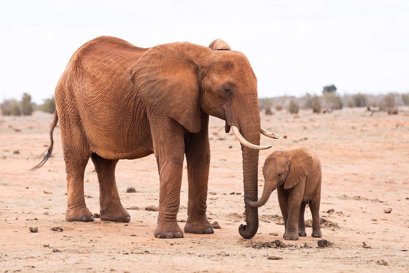
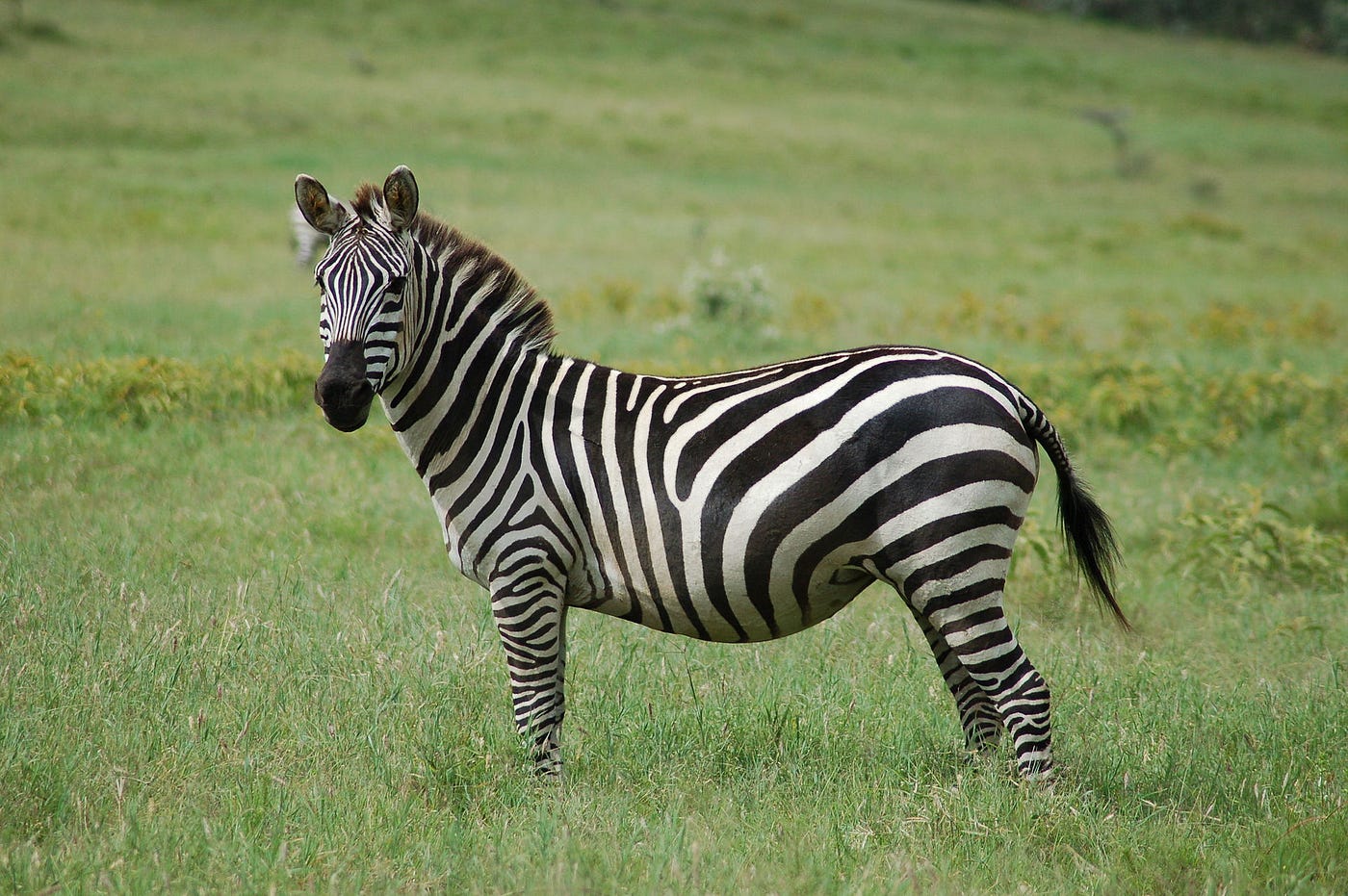
Test images :

### Import the YOLO module to load the fine-tuned model weights.
from ultralytics import YOLO

### Import OpenCV to handle saving and rendering the predicted visual outputs.
import cv2

### Import NumPy to perform any array manipulations on image pixels if needed.
import numpy as np

### Define the path to your optimized best performing training weights file.
weights_file = "d:/temp/models/african-wildlife-detection/My-Model-yolo26m/weights/best.pt"

### Load the optimized weights file into memory to begin predictions.
model = YOLO(weights_file) 

### Define the first test image path for inference testing.
imgPath1 = "Best-Object-Detection-models/YOLO26/How to detect African Wildlife animals using YoloV2026/Elephant2.jpg"

### Define the second test image path for inference testing.
imgPath2 = "Best-Object-Detection-models/YOLO26/How to detect African Wildlife animals using YoloV2026/Zebra_test.jpg"

### Execute inference on both image files simultaneously to generate predictions.
results = model.predict([imgPath1,imgPath2]) 

### Pull the complete dictionary of original class names from the model results.
names_dict = results[0].names

### Print the categories dictionary to verify valid label mapping.
print("Categories : ")
print(names_dict)

In summary, this inference code uses your best trained weights to analyze testing images and extract core detection metadata.

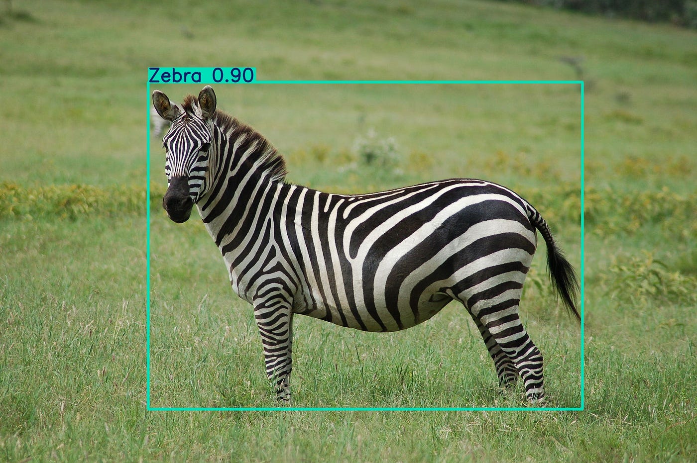
The Result :

Rendering Visual Annotations and Exporting Output

The final phase of our computer vision workflow extracts prediction details and saves annotated results to disk. Our Python code iterates through the inference results to access structural details like bounding boxes and classification probabilities. By converting this internal data into standard formats, you can easily use other libraries to draw on the original images.

The script converts the deep learning tensors into standard NumPy arrays for easy handling. This conversion makes it easy to map the numeric category IDs back to their original string labels. With these readable labels ready, OpenCV applies visual overlays directly onto the image pixels.

The code calls visualization tools to automatically render the bounding box frames over the detected wildlife targets. OpenCV then saves these modified images to disk, giving you a clear, permanent record of what the network discovered. Let us examine the Python loop that generates the visual outputs.

Why do we extract bounding box data as a separate NumPy array during the post-processing loop?

Extracting the tensor data into a standard NumPy array allows for easy compatibility with standard image processing libraries like OpenCV. This enables efficient post-processing and text annotation steps on the images without running into platform-specific issues.

### Loop through the prediction outputs to process and visualize each image individually.
for i, result in enumerate(results):

    ### Extract the bounding box coordinates from the inference predictions.
    boxes = result.boxes 

    ### Extract visual segmentation masks if available from your model output.
    masks = result.masks 

    ### Extract human pose keypoints if using specialized tracking configurations.
    keypoints = result.keypoints 

    ### Extract classification probabilities for high level classification results.
    probs = result.probs 

    ### Extract oriented bounding boxes for directional object detection tasks.
    obb = result.obb 

    ### Extract the class IDs as a standard NumPy array of integers.
    class_ids = result.boxes.cls.cpu().numpy().astype(int) 

    ### Print the predicted class IDs to confirm correct classification outputs.
    print("Predicted class Ids:", class_ids)

    ### Map the numerical class IDs back to their human-readable names.
    class_names = [names_dict[class_id] for class_id in class_ids]

    ### Print the exact names of detected classes found within the frame.
    print("Predicted class names:", class_names)

    ### Draw the visual bounding box overlays onto the original raw image.
    annotated_frame = result.plot()

    ### Save the processed image with bounding boxes to disk using OpenCV.
    cv2.imwrite(f"Best-Object-Detection-models/YOLO26/How to detect African Wildlife animals using YoloV2026/output_image_{i}.jpg", annotated_frame)

    ### Display the interactive window showing prediction results on screen.
    result.show()

In summary, this processing loop takes predicted animal coordinates, draws bounding boxes on the frames, and saves the images to disk.

Conclusion

Building a custom African wildlife detection YOLO model provides practical experience that balances machine learning theory with production execution.

Isolating your workspace dependencies with Conda ensures your system remains clean and avoids driver conflicts.

Following the entire pipeline — from environment setup and YAML creation to running the training loop — gives you a solid blueprint for any object detection task.

These reliable workflows allow you to expand the model’s capabilities, add more target classes, or deploy automated detection pipelines to edge devices.

FAQ

Q: Why should I train my YOLO model for 200 epochs?

A: Training for 200 epochs gives the model ample time to identify subtle features within the dataset while using patience triggers to stop early if performance levels off.

This strikes a careful balance between underfitting and overheating your compute resources.

Q: What does CUDA 12.8 add to the YOLO training process?

A: Using CUDA 12.8 enables modern hardware optimizations on NVIDIA graphics chips, resulting in significantly faster matrix multiplications.

This reduces total training times from hours down to just a few minutes.

Q: How do I prevent my model from overfitting to the background of training images?

A: You can use diverse images from different locations and times of day to force the model to identify specific animal features.

Adding varied imagery prevents the algorithm from relying on background colors to predict animal classes.

Q: Do I need a massive graphics processing unit to run this inference code?

A: No, running inference requires very low computational overhead compared to the heavy training step.

You can perform fast inference using a consumer CPU, though a dedicated GPU will make processing video feeds even faster.

Q: Why does the script use early stopping patience settings?

A: Patience halts training when the validation loss stops dropping for a specified number of consecutive epochs.

This keeps your model from memorizing the specific training images instead of generalizing effectively.

Q: What is the purpose of the config.yaml file?

A: The YAML file tells the algorithm where the training, testing, and validation folders live on your computer.

It also maps the specific numerical class IDs to their corresponding human-readable animal names.

Q: Can I add more than four classes to this wildlife detection model?

A: Yes, you can add dozens of classes by expanding your labels and updating the YAML configuration file.

Just ensure that each new class has enough annotated training images to allow the network to learn its distinct shapes.

Q: Why do we convert PyTorch tensor class IDs to NumPy arrays during inference post-processing?

A: PyTorch tensors are stored in GPU memory, while standard plotting tools like OpenCV expect regular CPU memory arrays.

Converting tensors into NumPy arrays makes drawing bounding boxes and labels simple and efficient.

Q: What does the imgsz=640 parameter control?

A: This sets the training image resolution to a standard size of $640 \times 640$ pixels.

Standardizing image dimensions balances fast processing times with detailed object visibility.

Q: How can I use this code to process custom videos instead of photos?

A: You can pass a video file path directly to the predict method instead of an image path.

The model will process the video frame-by-frame, applying your custom bounding box overlays in real time.

Connect

☕ Buy me a coffee — https://ko-fi.com/eranfeit

🖥️ Email : feitgemel@gmail.com

🌐 https://eranfeit.net

🤝 Fiverr : https://www.fiverr.com/s/mB3Pbb

Enjoy,

Eran