Math for AI: No PhD Required 🧮
By Muhammad Ishfaq | AI & ML Undergraduate | Computer Vision Builder
Math for AI: No PhD Required 🧮
By Muhammad Ishfaq | AI & ML Undergraduate | Computer Vision Builder
“You don’t need to be a mathematician to do AI. You need to understand what the math is doing — and why.”
😰 The Fear is Real — But It’s Lying to You
Let me be honest with you.
When I first started AI, I opened a deep learning paper and saw equations like:
$$\frac{\partial L}{\partial w} = \frac{1}{n} \sum_{i=1}^{n} (ŷ_i — y_i) \cdot x_i$$
I closed the tab immediately.
But here’s what nobody tells beginners: you don’t need to derive these equations from scratch. You need to understand what they mean and why they exist. There’s a huge difference.
This article covers the 4 math pillars of AI — Linear Algebra, Calculus, Probability, and Statistics — explained the way I wish someone had explained them to me: with intuition first, formulas second.
Let’s go.
📐 Part 1: Linear Algebra — The Language of Data
Linear algebra is how AI stores and transforms data. Every image, every word, every data point in your model is a number living inside a mathematical structure called a vector or a matrix.
Scalars, Vectors, and Matrices
Think of it as levels of complexity:
Scalar  →  a single number           →  accuracy = 0.91
Vector  →  a list of numbers         →  pixel row = [255, 128, 0, 200]
Matrix  →  a grid of numbers         →  grayscale image = 480×640 grid
Tensor  →  many matrices stacked     →  color video = frames × H × W × 3
import numpy as npscalar = 0.91 # just a numbervector = np.array([255, 128, 0, 200]) # 1D — one row of pixels
print(vector.shape) # (4,)matrix = np.zeros((480, 640)) # 2D — a grayscale image
print(matrix.shape) # (480, 640)tensor = np.zeros((30, 480, 640, 3)) # 4D — 30 frames of RGB video
print(tensor.shape) # (30, 480, 640, 3)Real AI connection: When my emotion detection system reads a webcam frame, that image becomes a tensor of shape (1, 48, 48, 1) — 1 image, 48×48 pixels, 1 grayscale channel. The entire neural network is just math operations on that tensor.
Vector Operations
Vectors can be added, scaled, and compared. These simple operations power everything in AI.
a = np.array([1, 2, 3])
b = np.array([4, 5, 6])
# Addition — combine features
print(a + b) # [5, 7, 9]# Scalar multiplication — scale a feature
print(a * 3) # [3, 6, 9]# Dot product — THE most important operation in AI
dot = np.dot(a, b)
print(dot) # 1×4 + 2×5 + 3×6 = 32What is a dot product intuitively?
It measures similarity. Two vectors pointing in the same direction have a high dot product. Two pointing in opposite directions have a negative one. In AI, this is how attention mechanisms in transformers measure “how relevant is this word to that word.”
Matrix Multiplication — The Heart of Neural Networks
Every layer of a neural network is a matrix multiplication. This is not an exaggeration — it is literally all that’s happening.
# Input: 1 sample with 3 features
X = np.array([[1, 2, 3]])          # shape: (1, 3)
# Weights: connecting 3 inputs to 4 neurons
W = np.random.randn(3, 4) # shape: (3, 4)# Forward pass through one layer
output = np.dot(X, W) # shape: (1, 4)
print(output.shape) # (1, 4) — 4 neuron outputsWhen you hear “a 512-neuron dense layer,” that means a matrix of shape (input_size, 512) is being multiplied with your data. That's it.
Norms — Measuring Size and Distance
v = np.array([3, 4])# L2 norm (Euclidean distance from origin)
norm = np.linalg.norm(v)
print(norm) # 5.0 (because √(3² + 4²) = √25 = 5)Norms appear everywhere in AI — in loss functions, regularization (L1/L2), and measuring how far predictions are from ground truth.
📈 Part 2: Calculus — How AI Actually Learns
If linear algebra is how AI stores data, calculus is how AI learns from mistakes.
The key concept: gradient descent. The key tool to understand it: derivatives.
Derivatives — The Rate of Change
A derivative tells you: if I change this input a tiny bit, how much does the output change?
f(x) = x²f'(x) = 2x ← the derivativeAt x = 3: f'(3) = 6 → output increases 6× faster than input
At x = 0: f'(0) = 0 → output is flat here (this is a minimum!)In AI: your loss function (how wrong your model is) depends on millions of weights. The derivative tells you which direction to adjust each weight to reduce the loss. That’s learning.
Gradient Descent — Learning Visually
Imagine you’re blindfolded on a hilly landscape. Your goal is to reach the lowest valley (minimum loss). You can’t see the whole map. But you can feel the slope under your feet.
Gradient descent says: at every step, feel the slope, then take a small step downhill.
# Simple gradient descent example
# Goal: minimize f(x) = x² (minimum is at x = 0)
def f(x):
return x ** 2def gradient(x):
return 2 * x # derivative of x²x = 10.0 # start far from minimum
learning_rate = 0.1 # step sizefor step in range(20):
grad = gradient(x) # which direction is downhill?
x = x - learning_rate * grad # take a step
loss = f(x)
print(f"Step {step+1:2d} | x = {x:6.3f} | loss = {loss:.4f}")Output (first few lines):
Step  1 | x =  8.000 | loss = 64.0000
Step  2 | x =  6.400 | loss = 40.9600
Step  3 | x =  5.120 | loss = 26.2144
...
Step 20 | x =  0.115 | loss = 0.0132
The model is finding the minimum — automatically. This is exactly what happens when you call model.fit() in TensorFlow or PyTorch. Millions of weights, same idea.
The Chain Rule — How Backpropagation Works
Neural networks have many layers stacked on top of each other. To train them, you need to calculate how the loss changes with respect to weights in every layer — even the deepest ones.
The chain rule lets you do this:
If y = f(g(x))
Then dy/dx = f'(g(x)) × g'(x)
In plain English: to find how a change in x affects y, multiply the local slopes layer by layer.
This is called backpropagation. Every deep learning framework (TensorFlow, PyTorch) implements this automatically. You just call loss.backward() and it computes all gradients for you.
Understanding this means you know why training works — not just that it does.
Learning Rate — The Most Important Hyperparameter
# Too large → overshoots the minimum (model diverges)
learning_rate = 10.0   # dangerous
# Too small → takes forever to converge
learning_rate = 0.0001 # very slow# Just right → converges smoothly
learning_rate = 0.001 # typical starting pointThis is why tuning the learning rate is the first thing every ML engineer does when a model isn’t training well.
🎲 Part 3: Probability — AI Thinks in Likelihoods
AI models almost never output “this IS a cat.” They output “this is 94.3% likely to be a cat.” That’s probability.
Basic Probability
# Probability: always between 0 and 1
P_rain    = 0.70   # 70% chance of rain
P_no_rain = 0.30   # 30% chance of no rain
# All outcomes must sum to 1
print(P_rain + P_no_rain) # 1.0 ✅# Probability of two independent events both happening
P_rain_monday = 0.7
P_rain_tuesday = 0.4
P_both = P_rain_monday * P_rain_tuesday
print(P_both) # 0.28 → 28%Conditional Probability — The Foundation of Smart AI
P(A | B) means: “What is the probability of A, given that B has already happened?”
P(spam | contains "FREE MONEY") = 0.97In words: given that an email contains "FREE MONEY",
there is a 97% chance it's spam.This thinking is inside every spam filter, medical diagnosis AI, and recommendation system.
Softmax — How Classifiers Output Probabilities
When your model classifies an image into categories, the final layer uses softmax to turn raw scores into probabilities:
import numpy as npdef softmax(scores):
exp_scores = np.exp(scores)
return exp_scores / np.sum(exp_scores)# Raw scores from the last layer of a neural network
raw_scores = np.array([2.1, 0.5, -1.2, 3.8, 0.9])
# (representing 5 emotion classes: angry, disgust, fear, happy, sad)probabilities = softmax(raw_scores)
print(np.round(probabilities, 3))
# [0.068 0.014 0.003 0.837 0.021 ...]
# Model is 83.7% confident this is "happy"print(f"Predicted class: {np.argmax(probabilities)}") # 3 → happyIn my emotion detection system, this is exactly what runs on every webcam frame.
Cross-Entropy Loss — Measuring How Wrong the Model Is
During training, we need to measure how far the model’s probabilities are from the correct answer. Cross-entropy loss does this:
def cross_entropy_loss(true_label, predicted_probs):
    return -np.log(predicted_probs[true_label])
# Model predicted: [0.1, 0.2, 0.7] for classes [cat, dog, bird]
# True label: 2 (bird)
predicted = np.array([0.1, 0.2, 0.7])
true_class = 2loss = cross_entropy_loss(true_class, predicted)
print(f"Loss: {loss:.4f}") # 0.3567 — lower is better# If model predicted correctly with high confidence:
predicted_good = np.array([0.01, 0.01, 0.98])
loss_good = cross_entropy_loss(2, predicted_good)
print(f"Good loss: {loss_good:.4f}") # 0.0202 — much lower!Lower loss = better model. The optimizer uses gradient descent to minimize this loss. Everything connects.
📊 Part 4: Statistics — Understanding Your Data
Before training any model, you need to understand your data. Statistics is the toolkit for that.
Measures of Center and Spread
import numpy as npexam_scores = np.array([55, 72, 68, 91, 45, 88, 76, 63, 95, 70])print(f"Mean: {np.mean(exam_scores):.1f}") # average: 72.3
print(f"Median: {np.median(exam_scores):.1f}") # middle value: 71.0
print(f"Std: {np.std(exam_scores):.1f}") # spread: 15.4
print(f"Min: {np.min(exam_scores)}") # 45
print(f"Max: {np.max(exam_scores)}") # 95Why this matters in AI:
- Mean — used in normalization
- Standard deviation — tells you how spread out your data is
- Min/Max — used in min-max scaling before training
Normalization — Preparing Data for Models
Neural networks train much better when all features are on the same scale. Two techniques:
data = np.array([200, 450, 100, 800, 350])# Min-Max normalization → scales to [0, 1]
normalized = (data - data.min()) / (data.max() - data.min())
print(np.round(normalized, 3))
# [0.143 0.5 0.0 1.0 0.357]# Z-score standardization → mean=0, std=1
standardized = (data - data.mean()) / data.std()
print(np.round(standardized, 3))
# [-0.6 0.4 -1.0 1.6 0.1 ]Always normalize your data before training. Without it, features with large values dominate the training and your model performs poorly.
Distributions — What Does Your Data Look Like?
import numpy as np# Normal (Gaussian) distribution — the most common in nature
# Mean=0, Std=1 → the standard bell curve
samples = np.random.normal(loc=0, scale=1, size=1000)
print(f"Mean: {np.mean(samples):.2f}") # ≈ 0.0
print(f"Std: {np.std(samples):.2f}") # ≈ 1.0Normal distributions appear in:
- Weight initialization in neural networks
- Noise modeling
- Assumption in many classical ML algorithms
Correlation — Finding Relationships
import numpy as npstudy_hours = np.array([1, 2, 3, 4, 5, 6, 7, 8])
exam_scores = np.array([45, 55, 60, 68, 75, 82, 88, 95])correlation = np.corrcoef(study_hours, exam_scores)[0, 1]
print(f"Correlation: {correlation:.3f}") # 0.997# Interpretation:
# +1.0 → perfect positive correlation
# 0.0 → no relationship
# -1.0 → perfect negative correlationIn ML, you use correlation to find which features are most useful for prediction and which are redundant.
Train/Test Split — The Golden Rule of ML
import numpy as npdataset_size = 1000
indices = np.arange(dataset_size)
np.random.shuffle(indices)split = int(0.8 * dataset_size) # 80% train, 20% testtrain_indices = indices[:split] # 800 samples
test_indices = indices[split:] # 200 samplesprint(f"Training samples: {len(train_indices)}") # 800
print(f"Testing samples: {len(test_indices)}") # 200Why this matters: You never evaluate your model on data it trained on — that’s cheating. The test set simulates real-world data the model has never seen. This is how you know if your model actually works.
🧩 Putting It All Together
Here’s how all 4 pillars connect inside one neural network training step:
1. LINEAR ALGEBRA
   Input data (tensor) → matrix multiply with weights
   → produces raw scores
2. CALCULUS
Compare scores to true labels using loss function
→ compute gradients (backpropagation)
→ update weights with gradient descent3. PROBABILITY
Convert raw scores to probabilities (softmax)
→ measure confidence of predictions
→ cross-entropy loss for training signal4. STATISTICS
Normalize input data before training
→ track mean loss and accuracy per epoch
→ evaluate model on held-out test setEvery single time you call model.fit(), this cycle runs thousands of times. Now you know what's actually happening inside.
📚 Your Math Checklist
✅ Scalars, vectors, matrices, tensors
✅ Dot product and matrix multiplication
✅ What a derivative means
✅ Gradient descent — step by step
✅ The chain rule and backpropagation
✅ Learning rate intuition
✅ Probability basics and softmax
✅ Cross-entropy loss
✅ Mean, median, standard deviation
✅ Normalization and standardization
✅ Correlation
✅ Train/test split
🎯 What’s Next?
Next Topic Why It Matters Supervised Learning Apply this math to real ML models Scikit-learn Build models without writing equations Matplotlib Visualize your data and training curves Neural Networks See all 4 pillars working together
💭 My Honest Advice
You don’t need to master all of this before building AI projects. I didn’t.
Start building. When something doesn’t work, come back to the math. You’ll understand it 10× faster when you have real context for why it matters.
The best way to learn math for AI is backwards — see the result first, understand the math after.
🔗 About the Author
Muhammad Ishfaq is an AI & ML undergraduate from Peshawar, Pakistan, building computer vision systems including real-time emotion detection, face recognition attendance, and AI interview monitors.
🔗 GitHub: github.com/CodewithnawaB 🔗 LinkedIn: linkedin.com/in/muhammad-ishfaq-842937310
Found this helpful? Drop a clap 👏 and follow — next up: Machine Learning basics.
Tags: Math AI Machine Learning Linear Algebra Calculus Statistics Probability Deep Learning Beginner Student Python Data Science
메타데이터
- post_id
- 9c5ffdfc2e95
- slug
- math-for-ai-no-phd-required-9c5ffdfc2e95
- url
- https://medium.com/@mishfa682/math-for-ai-no-phd-required-9c5ffdfc2e95
- canonical_url
- https://medium.com/@mishfa682/math-for-ai-no-phd-required-9c5ffdfc2e95
- author_url
- https://medium.com/@mishfa682
- status
- ok
- fetched_at
- 2026-07-18 23:42:34