Deutsch’s Algorithm

When I started my professional journey into Quantum Computing and Quantum algorithms design, Deutsch’s algorithm was the first one I learned. To be honest, the first time I read about it, it did not resonate with me. My first question was what is this algorithm about? Why is this so important to spend my time? These questions arise partially because at that time I did not understand that scientists in the quantum computing domain ask questions differently — I understood it over time by gaining more experience and observing how the quantum computing field evolves. Secondly, 4-5 years back from now, there were not many tutorials to frame quantum computing concepts in simple words. Finally, when I started my journey in the field, I was driven by all these buzzwords such as quantum speed up, quantum supremacy, etc. However, when I interacted with Deutsch’s algorithm, my first reaction was that it was far away from being practical in solving real-world problems. Recently, this algorithm emerged back in my academic discussions and inspired me to craft this post. While Deutsch’s algorithm does not find its application in solving real-world problems, it is one of the simplest algorithms to get your hands dirty and test your knowledge of quantum gates, qubits, and tensor products in practice. Additionally, Deutsch’s algorithm should give you a sense of how scientists in the quantum domain frame their questions.

Prerequisites. Tensor product, quantum gates.

Constant & Balanced Functions

Before jumping to Deutsch’s algorithm, let’s discuss the concept of the constant and balanced functions. If a function f(x) produces the same output regardless of the value of the input x, such a function is called a constant function.

For example, for the following test inputs f(1) = 8, f(-2) = 8, f(-10) = 8, f(10000) = 8 and so on, for any input x, the function always outputs 8.

For the purposes of Deutsch’s algorithm, we have to limit ourselves to a binary version of the constant function — the function’s input and output can be either 0 or 1. For example, regardless of the input value, the output is always 0 or always 1: f(0) = 1, f(1) = 1 or f(0) = 0, f(1) = 0.

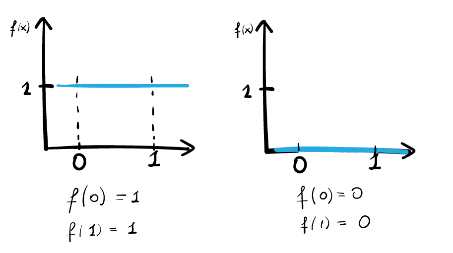
Graphs for the constant functions.

On the contrary, a balanced function f(x) gives different results for the different input values x. f(1) = 8, f( — 2) = 6, f( — 10) = 20, f(10000) = — 30 is an example of a balanced function. Again, if we want to work with bits, for a balanced function we get f(1) ≠ f(0). Or a more detailed example f(0) = 1, f(1) = 0 or f(0) = 0, f(1) = 1.

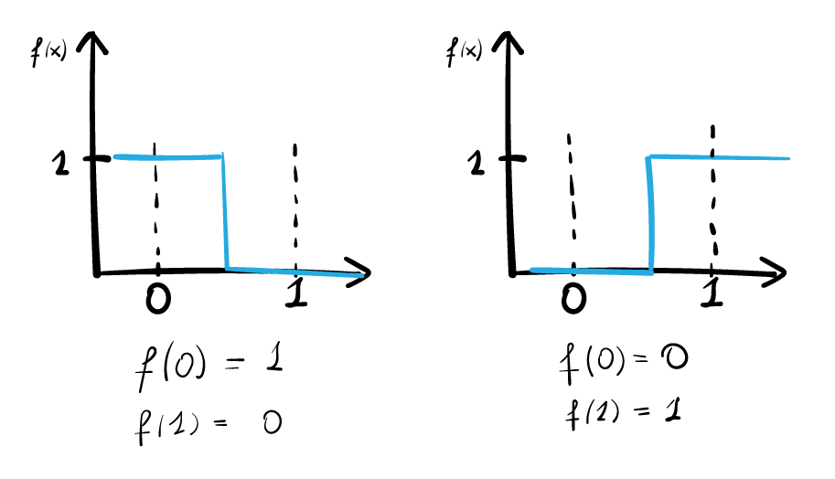
Graphs for the balanced functions.

Formally, we can say that we will work with a function that maps a bit of information to a bit of information:

Motivation and Problem Formulation

In short, I always think about Deutsch’s algorithm as the algorithm that can classify a function f(x) as a constant or a balanced function.

Let’s say someone gave me a black-box function f(x) where I have no idea how this function behaves, but I want to learn more about this function. Let’s assume that the only information that I know about it is that the function is binary. One example of how I can learn about this function is to classify it as a constant or balanced. To do so, I have to test my function for different inputs. Let’s say I will send 0 first — f(0). As the output, I can get either 0 or 1 which does not tell me much about my function. So, I have to send one more input, 1 this time — f(1). Again, as my output, I can get 0 or 1. If the outputs of both tests are equal, both 0’s or both 1’s, I can conclude that the function is constant. If the outputs of my tests are different, then the function is balanced. The chart below summarizes the classification flow.

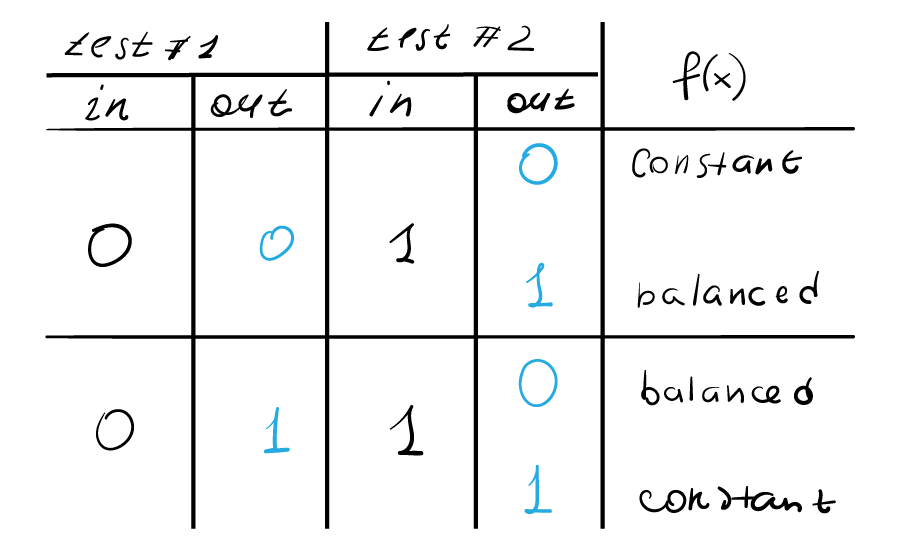
The important conclusion is that two tests are required to classify a function.

If you find the classification of a binary function confusing, I have an alternative explanation. Imagine I have a bag with two types of coins — silver and gold — and I want to classify the bag as either constant or balanced. A bag can contain either coins of one type or both types. To label my bag, I draw coins twice. If I draw two silver coins or two gold coins, the bag is classified as constant. If I draw one silver and one gold coin, in any order, the bag is classified as balanced.

David Deutsch, hence the name of the algorithm, proposed a quantum algorithm that can classify a function as balanced or constant in just one test. So, using Deutsch’s algorithm and a quantum computer I will do less work in achieving the same result!

Deutsch’s Algorithm

David Deutsch has shown how to classify a function, or a bag with coins if you wish, in one test only using a quantum computer. Here, I will go over the steps of the algorithm along with the mathematical justifications. If you feel uncomfortable working with the tensor product in quantum algorithms, please check out my previous blog tutorials.

Quantum circuit for Deutsch’s algorithm.

Step1. Prepare one qubit in |0> state and the second in |1> state. The quantum state for this two-qubit system is

Step2. Apply Hadamard gates to both qubits. The H gates bring the state of the two qubits into an equal superposition:

Step3. Apply a unitary U_f that represents the function we want to classify. Usually, this unitary is called an oracle and is assumed to be given to us. In practice, we have to construct it somehow and then apply it to a quantum circuit in a form of a unitary. The unitary acts in such a way that it applies a logical XOR operation to the second qubit where ⊕ means a direct sum or a logical XOR operator:

After we have applied the oracle, the state of the quantum circuit represents a superposition over all possible inputs to the function f(x). Because we have a binary function, we have a combination of two inputs only.

Now, the following part gets more involved. But that is the part where magic is going to happen!

A quantum computer knows if the function is balanced or constant at once, but we have to do a little bit work to understand how it classifies a function. Assume, that f(x) is constant, and let’s say that f(0) = f(1) = 1. Then,

Similarly, one can arrive at

for f(0) = f(1) = 0.

If we assume that that f(x) is balanced, and let’s say f(0) = 0 and f(1) = 1, then

Similarly, for f(0) = 1 and f(1) = 0,

Step4. We now apply the Hadamard gates on two qubits again:

Finally, after the measurement of the first qubit, we discover it either to be (±)0 and conclude that the test function is a constant or (±)1 which implies the function is balanced.

Note that (±) represents a global phase, the information that we lose at the moment of the measurement. Hence, in the end, the first qubit is either logical 0 or logical 1.

Deutsch’s algorithm demonstrates that testing a function just once is sufficient to classify it completely as either constant or balanced. This algorithm aims to demonstrate that a quantum computer can be more powerful over a conventional one in certain settings and tasks.

All opinions and views are my own and do not reflect opinions of my current, past, or future employers.

If you like my stories, please clap 👏(lots!!), leave a comment ✋, share, follow me 🔔, or buy me a cup of boba tea🧋.

Subscribe to my Substack feed on Quantum Computing!