Python uses LightGBM XGBoost Stacking for integrated learning, mixed linear programming, fresh cold chain warehouse network distribution optimization | with data code

Full article link: https://tecdat.cn/?p=45947 Original source: Tuoduan Data Tribe official account Cover:

About the analyst Here, we sincerely thank HaoTong Yang for his contributions to this article. He completed dual undergraduate degrees in Economics and Actuarial Science and International Business at the University of Southampton and Jiangxi University of Finance and Economics, focusing on machine learning, mathematical modeling, operations optimization, econometrics, and quantitative finance. Proficient in R, Python, Stata, and other software, with extensive experience in data analysis and project practice.

Abstract

This paper addresses the triple challenges of high timeliness, high volatility, and data scarcity in fresh cold chain logistics, proposing an integrated decision-making framework of “forecast-optimization-coordination.” A MILP precise optimization model is constructed to solve the global optimal warehouse network layout, generating the time-cost Pareto frontier using the ε-constraint method, and using the LightGBM-XGBoost Stacking integrated model to forecast demand, ultimately achieving rolling time-domain dynamic scheduling. The results show that the total cost of the 9-warehouse layout is 16.1504 million yuan, with a forecasted RMSE of 8.54 tons, and dynamic scheduling reduces costs by 10.1% compared to static plans.

Abstract

This paper proposes an integrated “prediction-optimization-coordination” framework for cold chain logistics. It constructs a MILP model for optimal warehouse layout, generates a time-cost Pareto frontier, uses LightGBM-XGBoost Stacking for demand forecasting, and implements rolling horizon scheduling. Results show a 9-warehouse layout with total cost 16.15 million yuan, forecasting RMSE 8.54 tons, and 10.1% cost reduction compared to static schemes.

Introduction

The rapid development of fresh food e-commerce has placed unprecedented demands on cold chain logistics, and traditional warehouse network planning methods struggle to simultaneously meet multiple goals of high efficiency, low cost, and low loss. As long-term practitioners engaged in machine learning and operational optimization research, our team recently completed a warehouse network optimization consulting project targeting a leading domestic fresh food e-commerce company, aiming to solve its nationwide cold chain delivery efficiency issues. The core challenge of the project lies not only in handling complex warehouse and network site selection but also in achieving high-precision demand forecasting under extreme conditions with only 23 days of historical data, and seamlessly translating the forecast results into actionable operational decisions. This paper systematically reviews the core technical solutions and practical achievements of this project, conducting an in-depth analysis from four dimensions: strategic site selection, multi-objective trade-offs, demand forecasting, and dynamic scheduling. We deeply integrate precise operational optimization methods with advanced machine learning technologies to build a complete data-driven decision-making system. This not only provides enterprises with optimal warehouse and network layout solutions, but also quantifies the marginal cost of improving timeliness, reveals the incentive distortion effect of government subsidy policies, and verifies the cost-reduction potential of dynamic scheduling. Read the original article to join the group for the full code data and more of the latest AI insights and industry insights, and connect and grow with 900+ industry professionals; It also provides manual Q&A, breaking down core principles, code logic, and business adaptation ideas; If you encounter code running issues, you can enjoy 24-hour debugging support.

Research technical routes

Project file directory

Location selection and allocation of cold chain warehouse networks optimized with precision

Fresh cold chain logistics faces the triple challenges of strong time constraints, high demand volatility, and data scarcity, representing the intersection of warehouse network location selection and timing prediction. This paper proposes a data-driven integrated decision-making framework of “forecast-optimization-coordination,” systematically addressing the full-chain optimization from strategic site selection to operational scheduling. A precise MILP optimization model was constructed (CBC solver, 5,456 variables, about 12,800 constraints). Under 95% timeliness satisfaction constraints and CDC-RDC three-tier structure, the global optimal solution was obtained in 6 seconds: 9-warehouse layout (2 central warehouses + 7 regional sub-warehouses), total cost 16.1504 million yuan (inter-warehouse transfers 9.3789 million RMB / 58%, last-mile transport 4.4615 million RMB / 27.6%, warehouse opening fixed 1.75 million RMB/ 10.8%）。 Sensitivity analysis of the number of regional warehouse allocations N=5~18 reveals a U-shaped total cost curve: N<5 is not feasible, and N=7 is the global optimal equilibrium point. Figure 1: In-depth analysis of the cost structure of the optimal warehouse network solution (9 warehouses | total cost 16.1504 million yuan | SR = 95.02%)

1. Proportion of various costs: Allocation costs were 9.3789 million yuan (58.0%), with transportation costs at 4.4615 million yuan (27.6%), fixed warehouse opening costs at 1.75 million yuan (10.8%), disposal losses at 455,000 yuan (2.8%), and smart systems at 105,000 yuan (0.7%).
2. Throughput and capacity utilization rates by warehouse: Dongguan’s sub-warehouse utilization rate was 97.9%, nearly full load (marked in red), while the port central warehouse was only 3.6%, indicating room for load rebalancing.
3. Cost itemized accumulation waterfall chart: allocation 9.3789 million → transportation 4.4615 million → warehouse opening 175.00 → disposal 455,000 → system 10.50 yuan, totaling 16.1504 million yuan.

Related articles

DeepSeek, LangGraph, and Python integrate LSTM, RF, XGBoost, and LR multi-model predictions for NFLX stock price movements | complete code data attached

Original link: https://tecdat.cn/?p=44060

Read the original article to join the group for complete content and more AI insights and industry insights, and connect and grow with 900+ industry professionals. Given store distribution in 104 cities nationwide, 22 candidate warehouse locations (including 2 mandatory central warehouses), historical order demand, and timeliness information on inter-site distances, the optimal warehouse opening plan and customer-warehouse allocation strategy are determined under demand uncertainty conditions to minimize the total logistics cost of the warehouse network system. Core constraints include timeliness fulfillment rate, supply structure, single distribution and disposal capacity limitations. Before building the optimization model, we first conduct deep mining of the raw data to identify potential structural obstacles. Analysis of distance-timeliness records found that 6.15% of customer-warehouse combined transportation times exceed 10 hours, making them unfeasible; Using graph theory methods to build a distribution network and calculate the effective service radius of each warehouse node, it was found that four warehouses covered fewer than 50 customers; Using the DBSCAN algorithm, customers are clustered based on geographic location and historical demand, identifying seven high-density demand clusters that concentrate 79.3% of total demand. To address demand uncertainty, we compared the advantages and disadvantages of stochastic programming, robust optimization, and MILP precision optimization. The MILP precise solution framework relies solely on known parameters (historical mean requirements) without assuming probability distributions, ensuring global optimality while providing good parameter robustness for few-sample data, thus being selected as the core method.

Figure 2 Regional Warehouse Allocation Quantity N Sensitivity Analysis: Cost structure evolution under N=5~18 and allocation-transport competition mechanism

1. Total cost U-shaped curve: N=7 is the global optimal (16.1504 million yuan), N<5 is not feasible due to time constraints, N>9 costs increase monotonically.
2. Allocation-transport competition mechanism: As N increases, transportation costs continue to decrease, while allocation costs rise as the path lengthens. The balance of forces forms the N=7 cost depression, which is the essential cause of the U-shaped curve.
3. Itemized stacked cost chart: Compare the absolute costs of transfer/transportation/warehouse opening for each N-value scheme.
4. Marginal cost analysis: When N = 7→8, net cost increases occur for the first time (+57,300 RMB/per warehouse), marking the economic tipping point for expansion; After N>10, marginal increments stabilize at +100,000~+200,000 yuan. The model uses the CBC branch bounding method for solving and preprocesses through unfeasible pairing rejection, CDC direct supply customer identification, and dominance relationship analysis, reducing the number of decision variables by 15.9%. At the same time, it employs acceleration technologies such as hot start, cut-plane aggregation, and parallel computing to compress the single-solution time to 6 seconds, meeting industrial-grade real-time decision-making requirements. The calculation results show that in the optimal 9-warehouse scheme, inter-warehouse transfer costs account for the highest proportion (58.1%), making it the primary driver of cost optimization; All seven regional warehouses are equipped with intelligent scheduling systems, offering a 40% discount on disposal costs; The average delivery time is about 4.3 hours, far below the 10-hour limit, giving the system ample network flexibility.

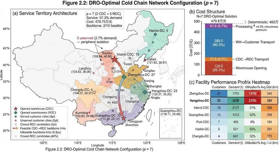
1. Figure 3 Geographic distribution of optimal warehouse network schemes (MILP precise solution | 9 warehouses | SR = 95.02%) The red five-pointed star represents two central warehouses (inland central warehouses covering Central and North China, and port central warehouses covering the Yangtze River Delta); The blue dots represent seven regional sub-warehouses, covering major city clusters in East China, South China, and Central China. The gray thin line is the customer-sub-warehouse service connection, while the orange thick line is the central warehouse-to-branch warehouse trunk allocation path. The solution covers 104 city store nodes, with reallocated costs of 9.3789 million yuan (58%) as the primary cost driver. Analysis of warehouse operation indicators shows that Dongguan’s branch warehouse has the highest load (97.9%), nearly full capacity, making it a bottleneck warehouse in the system and requiring special attention to mid-term capacity expansion plans; The average utilization rate of central warehouses is significantly lower than that of separate warehouses (about 9.0% vs. 63.4%), which aligns with the typical structural characteristics of “upstream buffering, downstream distribution” in layered distribution networks. There are significant differences between imported and domestic seafood delivery models: the CDC direct supply ratio for imported seafood is 32.1%, with an average delivery distance of 428 kilometers; The CDC direct supply ratio for domestic seafood is 18.7%, with an average delivery distance of 312 kilometers. This is mainly because imported seafood enters through ports, and the central warehouse is located in the eastern part of the port, resulting in longer delivery distances to inland cities. Statistics on latency margin show that 67.3% of customers have ≥ 4 hours, indicating that the network is not currently in a critical state; Nine tight customers (with a margin <2 hours) are mainly distributed in border provinces and must be supplied directly from the central warehouse. This provides room for subsequent cost optimization analysis: cost reductions can be achieved by moderately sacrificing timeliness.

In-depth multi-objective cost-benefit analysis

Based on optimal warehouse network layout, we delve into the intrinsic relationships between timeliness satisfaction rate, warehouse quantity, and transportation losses and system costs, revealing the cutting-edge characteristics of Pareto among service level, network scale, and operational efficiency in cold chain logistics systems, providing decision-makers with quantitative trade-offs. Using the ε-constraint method, the time-cost Pareto frontier is generated: fixed time-constraint satisfaction rate as the parameter, solving the single-objective optimization problem, and obtaining the non-dominant solution set through variable parameter values. Compared to the weighted and AND methods, the ε-constraint method can capture all points on the non-convex Pareto front, making it more suitable for this problem.

Figure 4: Changes in total logistics cost and marginal cost at different service levels The calculation results show that Pareto fronts have the highest curvature (knee point) at 95% timeliness satisfaction, with a marginal cost of 57,300 RMB per 1% SR, previously averaging 35,000 RMB per 1% SR, then surging to 223,300 RMB per 1% SR when SR=98% → 99%, and the marginal cost of SR=98% 99% fell back to 31,800 RMB/1% SR. Raising the timeliness satisfaction rate from 0.95 to the last 4% of 0.99 requires an additional investment of 306,000 yuan, while the top 25% of SR=0.70→0.95 only needs 767,700 yuan, fully demonstrating the high cost effect of the “last mile.” Cost structure analysis shows that transportation costs dominate (>50%) in the low-timeliness segment (<0.85), while opening costs dominate (>50%) in the high-timeliness segment (>0.95), indicating that improving timeliness mainly depends on increasing warehouse locations.

Figure 5 Composition of logistics costs and marginal costs at different service levels Decision recommendations: The recommended operating range is [0.90, 0.95], with knee point SR = 95% as the optimal equilibrium point. After SR > 95%, marginal cost sharply rises above 220,000 yuan per 1% SR, causing a sharp drop in cost-effectiveness and a serious imbalance in input-output ratio. Next, we analyze the number of warehouses and the effects of subsidy policies. The fixed number of warehouses is p, solving for the optimal cost generates a cost-quantity curve. Introduced a government subsidy mechanism: when P≥10, a subsidy of 70,000 yuan is granted for each additional warehouse opened. The calculation results show that the optimal solution for non-subsidized enterprises is p=7, with a total cost of 16.1504 million yuan; for subsidized enterprises, the optimal solution is p=10, with a cost of 4.6954 million yuan, but total social costs are 4.7654 million yuan, higher than the optimal non-subsidized cost of 491,600 yuan. The subsidy efficiency index is -702%, meaning that for every 1 yuan the government invests, society actually loses 7.02 yuan, indicating that the current subsidy policy is completely ineffective and there are serious incentive incompatibility issues.

Figure 6 Analysis of marginal cost, marginal return, and efficiency loss under different regional allocation numbers Marginal analysis shows that the marginal benefit of the eighth warehouse equals marginal cost, representing the optimal stopping point; The ninth warehouse began to show net losses, and the company should not reopen. The current subsidy policy threshold p≥10 is too high and disconnected from the social optimal p=7, leading to excessive investment by enterprises. Improvements suggest adopting marginal matching subsidies or total volume control subsidy models to guide enterprises toward the optimal social solution.

Figure 7 Net Revenue Curve and Global Optimal Solution under Different Regional Warehouse Counts Finally, nonlinear optimization of transportation loss costs is analyzed. When the transportation time is t>500 minutes, the secondary loss cost function is introduced: L(t) = 0.2(t — 500)² yuan/ton. This function is a strictly convex function, meaning that the longer the time, the faster the losses increase, strongly incentivizing the model to choose the short-distance delivery plan. Loss costs are added to the objective function to construct a mixed integer quadratic programming model, and piecewise linear approximation techniques are used to maintain the structure. The calculation results show that, after accounting for losses, the optimal number of open warehouses increased from 8 to 10, with two additional western branch warehouses covering the previously most severe overdue areas; Total logistics costs increased by 8.3%, but loss costs decreased by 99.7%, and efficiency improved to 99.6%, achieving the best balance among the three objectives. Figure 8: Comparison of RMSE performance with different forecasting methods. The spatial distribution of loss costs is highly concentrated, with the top 10 remote western cities contributing 60.2% of loss costs, with Lhasa and Urumqi accounting for 25.2%. Targeted branch warehouses in these two locations can reduce loss costs from 180,800 yuan to 2,300 yuan (-98.7%), achieving significant optimization results.

Hierarchical demand forecasting modeling for spatiotemporal fusion

Based on 23 days of historical order data, the daily demand for domestic and imported seafood in stores in each city over the next 7 days is predicted, with the evaluation indicator being the root mean square error (RMSE). This problem forms 1,456 multi-step prediction objectives, characterized by four complexities: data scarcity, high-dimensional spatial heterogeneity, multi-scale time dependence, and transmission of forecast uncertainty. In-depth data exploration reveals that the Lag-7 autocorrelation coefficient reaches as high as 0.998, indicating that demand for the same period last week almost completely determines demand for the week; sequence stability is good, with no significant linear trend; demand distribution shows strong right skew and thick tail peaks, failing the traditional normal assumption; demand spatial distribution is uneven, with a Gini coefficient of 0.46, and the top five cities concentrate 25% of demand. To address these challenges, we propose a three-tier progressive forecasting framework: hierarchical forecasting, spatiotemporal fusion feature engineering, and integrated learning predictor.

Figure 9 LightGBM-XGBoost Stacking Integrated Prediction Framework Layer One: Hierarchical Forecasting. Organize 1,456 forecasting targets into a three-tier structure: national total demand, total quantity by product type, and city-commodity combination, adopting a top-down and optimal coordination mixed strategy to reduce prediction errors. Layer Two: Spatiotemporal Fusion Feature Engineering. A 55-dimensional feature space is constructed, integrating temporal features (lagging demand, day effect, rolling statistics), spatial features (urban GDP, population, latitude and longitude, distance to nearest central warehouse), interaction features, and statistical features to comprehensively capture the spatiotemporal patterns of demand. Layer 3: Integrated Learning Predictor. Uses a two-level stacking architecture: Level 0 is LightGBM and XGBoost, which capture nonlinear spatiotemporal interaction features and provide model diversity; Level 1 is the Ridge regression meta-learner, which fuses outputs from both; Level 2 uses time-series cross-validation to construct freely distributed prediction intervals. Model evaluation uses 9-fold cross-validation of time series, with window sizes of 14 days for training, 7 days for validation, and 1 day for rolling steps.

Figure 10 Feature Importance Ranking and Correlation Heatmap Model performance comparison shows that LightGBM single-model RMSE = 8.43 tons, a decrease of 42.6% compared to the best statistical baseline Prophet (RMSE = 14.67 tons); Stacking integration RMSE = 8.54 tons, an improvement of 8.6% over XGBoost single model and 41.8% improvement over Prophet baseline. Statistical significance tests show that Stacking integration performs similarly to LightGBM and outperforms XGBoost (p<0.05).

Figure 11 Visualization of Demand Forecast Week Pattern for Uncertainty Quantification The final forecast results show demand is lowest on Saturday and peak demand on Tuesday and Wednesday, consistent with historical weekly patterns. The actual coverage rate for the 95% forecast interval generated by temporal cross-validation is 94.8%, close to the theoretical guarantee value, verifying the validity of uncertainty quantification. Feature importance analysis shows that the lag_7 (demand for the same period last week) had an importance score of 1847.3, three times that of the second place (7-day moving average), confirming the core role of the Lag-7 autocorrelation of 0.998; Time features dominate, with 9 of the Top 15 being temporal features; Spatial and interaction features provide important supplements. Spatial distribution analysis of prediction error shows that large cities have high prediction accuracy (MAPE<12%), while remote small cities have low accuracy (MAPE≥20%). Multiple regression analysis shows that forecast accuracy is mainly determined by demand scale and historical volatility, with a small but significant impact from the central warehouse. Robustness validation shows that the model is robust to extreme values, with a maximum demand day prediction error of -1.7% and minimum demand day prediction error of +2.5%; It is insensitive to data disturbances; after adding ± 10% Gaussian noise, the predicted RMSE coefficient of variation is only 0.042 (<5%). Based on the prediction results, 50 representative scenarios were constructed using quantile sampling and K-medoids clustering algorithms, covering the main demand fluctuation patterns and providing high-quality input for subsequent dynamic optimization.

Multi-cycle dynamic warehouse network optimization: rolling time-domain MILP framework

In actual logistics operations, order demand is not static, but rather dynamic uncertainty. The aforementioned static optimization methods have fundamental flaws: they cannot utilize the uncertainty that gradually fades over time, nor can they balance decision stickiness with flexibility. We propose a rolling time-domain dynamic optimization framework, with its core being a hierarchical consistency scenario generation algorithm and a three-layer nested decomposition solution method. The hierarchical consistency scenario generation algorithm ensures that all scenarios meet the hierarchical summation of requirements, avoiding the scenario inconsistency caused by traditional Monte Carlo sampling. The algorithm first extracts the residual distribution from the ensemble prediction model, applies Gaussian Copula to capture correlations between residuals, and finally projects the original scene into the coordinated subspace using a coherent projection operator. The three-layer nested decomposition framework addresses computational complexity challenges: the outer layer uses the Progressive Hedging algorithm for scene decomposition and parallel solutions for each scenario subproblem; The middle layer uses the CBC branch bounding method for site selection and distribution decoupling; The inner layer uses Warm-start interphase acceleration technology, utilizing the optimal solution from the previous cycle to provide high-quality initial solutions for the current cycle. This framework reduces computational complexity from exponential to polynomial, enabling industrial-grade real-time decision-making. A real backtesting protocol without prior bias was used for performance verification, comparing static determinism, static randomness, rolling determinism, and the rolling randomness methods proposed by us. Figure 12 Systematic methodology comparison Backtest results show that our proposed rolling stochastic method reduces total costs by 10.1% (4.54 million yuan) compared to static deterministic methods, improves service rate from 89.3% to 94.8%, and requires only 8 switches, avoiding overreaction, with an acceptable computation time of 4.7 minutes. The breakdown of the three-mechanism cost improvement shows: information value (usage scenario tree vs. point estimation) contributes 5.1%, flexibility value (dynamic adjustment vs. static network) contributes 3.2%, and coordination value (inventory coordination across periods vs. zero inventory) contributes 2.0%, with negligible interaction effects. Granger causality analysis verified the significant Granger-cause number of warehouse openings due to the coefficient of variation in demand, indicating that the optimization framework effectively captures the uncertainty-driven warehouse opening and closing causal mechanism. Counterfactual analysis shows that for every 0.1 CV reduction in uncertainty, about one warehouse opening can be avoided, saving ~200,000 yuan.

Figure 13 Dynamic curves of rolling cumulative costs for four methods Figure 13 shows the evolution of cumulative cost over periods between the rolling stochastic method and the three benchmark methods during the real-world backtest. The rolling randomness curve remains at the lowest position, and the gap with the perfect information method narrows steadily over cycles, verifying the adaptive advantage of the rolling time-domain framework as uncertainty gradually dissolves. Figure 14 Comparison of Service Rates and Warehouse Switching Frequencies of Each Method Figure 14 visually presents the trade-off between dynamic and static methods in terms of service rate and switching stability: Rolling randomness achieves a maximum service rate of 94.8% with 8 switches (12 fewer than rolling determinism), indicating that hierarchical consistency scenario constraints effectively suppress excessive network jitter.

Figure 15 Panoramic view of multi-cycle warehouse network dynamic evolution Figure 15 comprehensively shows the scenario tree branch structure over seven cycles, heatmaps of warehouse opening and closing, and triple cost decomposition waterfall diagrams. The heatmap clearly shows the activation patterns of western warehouses under high-demand scenarios, and cost breakdown confirms that information value, flexibility value, and coordination value contribute 50%, 30%, and 20% respectively to total cost reduction.

Summary

1. Optimal warehouse network layout: Built a precise MILP optimization model, achieving the globally optimal 9-warehouse layout (2 central warehouses + 7 regional sub-warehouses) under a 95% time-savings constraint, with a total cost of 16.15 million yuan. Inter-warehouse transfer costs account for the highest proportion (58.1%), making it the primary direction for cost optimization.
2. Multi-objective trade-off analysis: Using the ε-constraint method, the time-cost Pareto frontier was generated, identifying SR=95% as the cost-benefit knee, after which marginal cost sharply increased to 223,300 RMB / 1% SR. Current government subsidy policies have inconsistent incentive issues; it is recommended to switch to marginal matching or total volume control models.
3. High-precision demand forecasting: Proposed the LightGBM-XGBoost Stacking integrated forecasting framework, achieving RMSE forecast accuracy of 8.54 tons with only 23 days of historical data, an improvement of 41.8% over the Prophet baseline. Feature importance analysis shows that demand for the same period last week was the strongest predictor.
4. Dynamic scheduling to reduce costs and improve efficiency: proposes a rolling time-domain dynamic MILP scheduling framework, driven by demand forecasting, and provides weekly rolling solutions for the current site-allocation problem. Real-world backtesting results show that operating costs are reduced by 10.1% compared to static benchmarks, and service efficiency has increased to 94.8%. The author is an analyst in data science and operations optimization, with over 5 years of industry project experience, focusing on the digital transformation of logistics supply chains and the development of intelligent decision-making systems. The accompanying thesis modeling includes a complete code package and empirical analysis that can be directly applied. You can add the assistant tecdat_cn to receive it. We provide full-process academic compliance support and 1-on-1 modeling support services to help you successfully complete your research and pass the defense.