One Ton of Carbon

Climate change is becoming increasingly visible in everyday life. Heatwaves are disrupting cities, straining infrastructure, and making outdoor work more difficult. Food prices rise after droughts and floods, and erratic rainfall damage harvests across multiple regions at once. Water shortages increasingly affect agriculture, hydropower production, and local ecosystems, while wildfires, storms, and extreme rainfall events are becoming more frequent and destructive in many parts of the world.

At the same time, public awareness of climate change has expanded dramatically over recent decades. IPCC assessments, climate disclosure rules, carbon markets, expanding emissions reporting, and near-constant media coverage have pushed greenhouse gas accounting into mainstream political, economic, and public debate.

Each year, international organizations publish reports on emissions inventories and rankings. These numbers allow us to compare countries, sectors, and even companies, making climate performance appear measurable, comparable, and trackable over time. Yet despite the growing visibility of climate accounting, a basic misunderstanding still persists: most people do not fully understand what “one ton of emissions” actually imply. What we generally know is that more emissions are bad. But there is still widespread confusion between carbon dioxide (CO2), a specific greenhouse gas, and greenhouse gases more broadly. The terms are often used almost interchangeably, which is understandable because carbon dioxide is by far the largest contributor to human-caused warming in absolute terms.

But this simplification is misleading. Different greenhouse gases behave very differently in the atmosphere. They vary in how strongly they trap heat, how long they remain in the climate system, where they come from, and how they affect warming over time. A ton of carbon dioxide (CO2) can affect the climate for centuries. Methane (CH4), another GHG, creates intense warming over the short run before breaking down. Nitrous oxide (N2O) persists for more than a century. Some fluorinated gases (F-gases) trap thousands of times more heat than CO2 despite being emitted in tiny quantities.

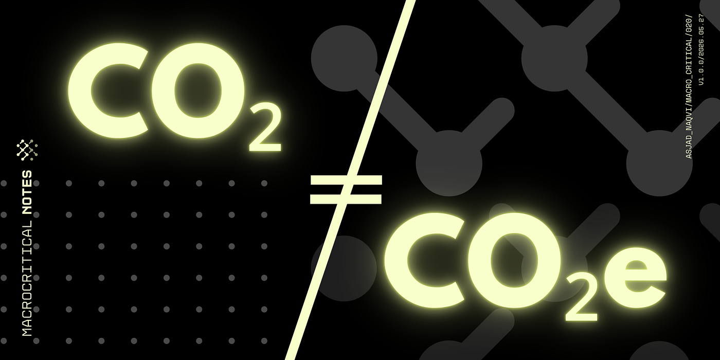
But we don’t see rankings of methane, nitrous oxides, or flourinated gases. We hear almost only about CO2 emissions. And that is because all the GHGs are converted into one common unit: carbon dioxide equivalent, or CO2e. And this is different from CO2.

CO2e is an accounting system designed to make climate reporting, regulation, and carbon markets possible. But it also hides how greenhouse gases differ fundamentally in how they are produced, how long they remain in the atmosphere, and how they drive warming.

Greenhouse Gases 101

Before we dive deeper in how to convert all GHGs into CO2e, lets do a brief recap of what GHGs are:

Earth receives incoming solar energy, absorbs part of it, and re-emits heat outward as infrared radiation. Greenhouse gases absorb some of that outgoing heat and re-radiate it, including back toward the surface. This natural greenhouse effect is essential for life and without it, the planet would be far colder. So essentially, GHGs are not the problem since they are needed to sustain life on this planet. It is the acceleration of GHGs in the atmosphere, or GHG concentration that is the main issue.

Human activity over the past 150 years, or since the industrial age, has intensified it at a speed that natural systems cannot easily absorb. We have, at scale, increased atmospheric heat-trapping gas concentrations through fossil fuel combustion, industrial processes, land-use change, and agriculture. Ever since the first IPCC report, the numbers are unambiguously clear about human impact. Before industrialization, atmospheric CO2 was around 280 parts per million. In 2025, it exceeded 426 ppm and continues to rise.

Source: Our World in Data: https://ourworldindata.org/grapher/co2-long-term-concentration

Global average temperature has risen roughly 1.3°C above pre-industrial levels. Furthermore, that warming is not evenly distributed. Some regions have warmed twice as fast and we are already observing the consequences: intensified heat waves, altered precipitation patterns, earlier snowmelt, shifting growing seasons, and destabilized ice sheets. This can lead to additional problems as critical non-reversible “tipping points” are crossed creating unintended and non-linear consequences.

The relationship between cumulative emissions and temperature is well-established. There is no threshold at which warming suddenly stops. Every tenth of a degree matters and the consequences of this increase are non-linear and complex. At 1.5°C above pre-industrial (the aspirational Paris target), some ecosystems and communities face acute risk. At 2°C, the risks compound. Beyond 2°C, the situation deteriorates rapidly. The carbon budget, or the total amount of CO2 humanity can still emit before exceeding a temperature target at a certain point in time, is finite and shrinking with every year of continued emissions.

The timeline is also critical. The warming already observed (1.3°C) reflects emissions from decades past. CO2 concentration does not warm the planet instantaneously but it’s impacts accumulate over decades. Even if emissions stopped today, the planet would continue warming for some time due to existing atmospheric gases and delayed climate system responses. This is called “committed” or “pipeline” warming. For methane and other short-lived gases, the lag is shorter. Cutting methane today can prevent additional warming within years. But for CO2, the commitment is measured in centuries.

The **IPCC synthesis** makes it clear that warming is unequivocal, human emissions are the dominant cause, and the rate of change is historically unprecedented. What makes this urgent for policy actors is that the warming drivers are already in the atmosphere. We are not deciding whether warming happens. Rather, we are deciding how much more warming we will add. That distinction changes everything about risk modeling, timing, and sequencing.

Types of Greenhouse Gases (GHGs)

Climate change is not caused by a single pollutant, but by a basket of greenhouse gases that differ significantly in origin, atmospheric behavior, and warming impact. International climate reporting under the United Nations Framework Convention on Climate Change (UNFCCC) therefore tracks multiple gases simultaneously through standardized inventory and transparency frameworks. More on the UNFCCC transparency framework here: https://unfccc.int/Transparency

Let’s briefly introduce the core GHGs:

CO2 is the main GHG. Fossil fuel combustion, cement production, and deforestation pour out CO2 at massive scale. It is not the most potent per unit, but sheer volume makes it dominate long-term warming. Once in the atmosphere, it lingers for centuries, accumulating with each year’s emissions.

Methane (CH4) comes from natural gas infrastructure leaks, coal mining, livestock digestion, rice cultivation, landfills, and decomposing organic waste. Per unit, it traps heat much more aggressively than CO2 over short time horizons. Unlike CO2, however, methane breaks down relatively quickly in the atmosphere. This makes methane especially important for near-term warming dynamics.

Nitrous oxide (N2O) is mainly associated with fertilizer use, agricultural soils, and manure management. It is less publicly discussed than CO2 or methane, but it is both highly potent and long-lived, remaining in the atmosphere for more than a century. Agricultural emissions therefore present a particularly difficult challenge because there are relatively few simple substitutes for fertilizer-intensive food production systems.

Fluorinated gases (HFCs, PFCs, SF6, etc.) are largely industrial gases used in refrigeration, electrical insulation, semiconductors, and electronics manufacturing. They are emitted in comparatively tiny quantities, but many trap thousands of times more heat than CO2. Some earlier generations of fluorinated gases were also linked to ozone depletion, which led to a separate global regulatory regime under the Montreal Protocol. More recently, international agreements such as the Kigali Amendment have sought to phase down highly potent refrigerants and replace them with lower-impact alternatives.

How do we translate different gases in one number

GHGs differ along two dimensions: first is warming intensity, or how much heat each unit traps relative to CO2. The second is atmospheric persistence, or how long it stays in the climate system before breaking down or being absorbed. Together, these characteristics determine whether a gas primarily affects short-term warming, long-term climate stabilization, or both. Once we understand these differences, it becomes much harder to think of emissions as interchangeable “tons of carbon.”

CO2-equivalent or CO2e is an accounting framework that helps us compare these incomparable gases. In order to do so, climate science uses a conversion factor called the **Global Warming Potential**, or GWP.

GWP compares how much warming each gas causes relative to CO2 over a chosen time window. CO2 is set to 1 by definition. Every other gas gets a number that reflects its intensity and persistence relative to that baseline.

The most widely used benchmark is GWP100, which simply asks:

If I emit one ton today, how much cumulative warming damage will it cause over the next hundred years compared to one ton of CO2?

And this is where it gets complicated. GWP values are not fixed. They are revised with each IPCC Assessment Report (ARs) as atmospheric chemistry and radiative forcing estimates, and climate modeling improves. The table below summarizes how key GWP values have changed across IPCC Assessment Reports 4, 5, and 6:

| Gas / Substance          | AR4    | AR5    | AR6     | Common sources / production                    |
|--------------------------|--------|--------|---------|------------------------------------------------|
| CO2                      | 1      | 1      | 1       | Fossil fuels, cement, deforestation            |
| Methane (CH4)(non-fossil)| 25     | 28     | 27.0    | Livestock, rice cultivation, landfills         |
| Methane (CH4)(fossil)    | –      | 30     | 29.8    | Oil & gas leaks, coal mining                   |
| Nitrous oxide (N2O)      | 298    | 265    | 273     | Fertilizers, agricultural soils                |
| Nitrogen trifluoride(NF3)| 17,200 | 16,100 | 17,400  | Semiconductor and electronics manufacturing    |
| Sulfur hexafluoride (SF6)| 22,800 | 23,500 | 24,300  | Electrical switchgear and transformers         |
| HFC-134a                 | 1,430  | 1,300  | 1,530   | Refrigeration and vehicle air conditioning     |
| PFC-14 (CF4)             | 7,390  | 6,630  | 7,380   | Aluminum smelting, semiconductors              |
| CFC-12                   | 10,900 | 10,200 | 12,500  | Older refrigeration systems                    |
| HFO-1234yf               | <1     | <1     | 0.501   | Modern low-GWP refrigerants                    |

Let’s briefly discuss this table: Fluorinated gases cluster at the extreme end where SF6 and NF3 carry warming potentials in the tens of thousands, meaning even small leaks carry outsized climate consequences. HFO-1234yf, a relatively new creation, illustrates how refrigerant chemistry has been redesigned to reduce warming impact while preserving function. Methane (CH4) values have been revised modestly upward from AR4 to AR5, then slightly down in AR6, reflecting improved modeling. Nitrous oxide values dropped from AR4 to AR5, a reminder that these numbers are scientific estimates subject to revision, not fixed physical constants. Currently most common reporting is done using AR5 values, or more specifically we use GWP100_AR5 benchmarks.

Under current (AR6-aligned) science, one ton of methane roughly equals 27–30 tons of CO2 on that hundred-year basis. That does not mean methane is “worse” in all contexts. Only that over a century, the cumulative heating effect is equivalent to releasing 27 tons of CO2. Over a 20-year window, the same ton of methane is closer to 80 tons CO2-equivalent, because methane’s heat-trapping is more aggressive upfront. But the methane breaks down, so by 100 years, the factor drops.

This conversion framework is what allows countries, factories, and corporations to aggregate very different gases into one comparable emissions inventory. It is also where climate accounting begins to diverge from the underlying physical reality of how different gases behave in the atmosphere.

The **Greenhouse Gas Protocol** is the world’s most widely used framework for measuring and reporting greenhouse gas emissions. Developed by the World Resources Institute (WRI) and the World Business Council for Sustainable Development (WBCSD), it provides standardized accounting rules that allow companies, governments, and organizations to calculate and compare emissions consistently. The Protocol underpins many corporate climate disclosures, ESG reports, carbon footprint calculations, and net-zero commitments, and operationalizes IPCC climate science into practical reporting standards. It is also widely known for its distinction between Scope 1, Scope 2, and Scope 3 emissions, which separate direct emissions from indirect electricity-related and supply-chain emissions.

The latest GHG Protocol guidance:

[embed]

The interactive visualization below shows how total greenhouse gas emissions are composed across sectors and gases using CO2-equivalent accounting. While sectors such as power generation, transport, buildings, and industrial combustion are still overwhelmingly dominated by CO2 emissions, other sectors reveal a very different composition. Agriculture is driven largely by methane (CH4) and nitrous oxide (N2O), reflecting livestock production and fertilizer use, while industrial processes and fuel extraction contain important contributions from fluorinated gases and methane leaks. The data are based on the Emissions Database for Global Atmospheric Research 2025 report and use GWP100 values from the IPCC Fifth Assessment Report (AR5), which remain the benchmark in many international reporting systems and emissions inventories.

[embed]Full screen version: https://public.flourish.studio/visualisation/29120039/

Two factories: same CO2e, different inventories

Imagine two factories in Europe that each report annual emissions of 100 tons CO2e. At first, they appear identical in climate accounting. But their actual emissions profiles are very different.

Factory A emits almost entirely CO2 from fossil fuel combustion used for boilers, furnaces, and industrial heat. Its climate profile is dominated by long-lived carbon emissions tied directly to energy use.

Factory B also reports 100 tons CO2e, but a large share comes from methane leaks and fluorinated gases used in refrigeration and industrial equipment. Although its total CO2e is the same, the composition of emissions is fundamentally different.

Factory A primarily falls under carbon-pricing systems such as the EU Emissions Trading System (EU ETS), where compliance mainly depends on reducing fossil fuel combustion. Factory B faces a more fragmented regulatory landscape. Methane emissions increasingly fall under methane monitoring and leak detection rules, while fluorinated gases are governed by separate EU F-gas regulations and refrigerant phase-down policies.

The climate effects also differ substantially. Since methane creates intense near-term warming while CO2 accumulates over centuries locking in long-term warming, the two facilities with identical annual CO2e emissions can contribute very differently to short-term warming pressure, long-term climate stabilization, and future policy risks.

Yet in many emissions inventories, sustainability reports, and climate rankings, both factories appear as the same number with 100 tons CO2e.

Why the time horizon matters in the climate story

Global Warming Potential (GWP) is most commonly measured over a 100-year horizon, known as GWP100. But this is not a scientific choice but rather a policy convention. Using a 100-year timeframe creates a relatively stable and standardized basis for comparing greenhouse gases across countries, sectors, and reporting systems. It smooths out some of the extreme short-term differences between gases and makes long-run climate accounting more manageable.

But the choice of time horizon also shapes climate policy itself. A shorter timeframe would place much greater emphasis on gases such as methane, whose warming impact is extremely strong in the near term. A longer timeframe places more weight on the cumulative effects of CO2, which persists in the atmosphere for centuries.

The 100-year benchmark therefore represents, to some extent, a compromise between atmospheric physics and policy practicality. It allows governments and industries more time to adapt and transition away from carbon-intensive systems. Policymakers are often concerned that excessively abrupt transitions could trigger broader economic disruptions, including energy price shocks, stranded assets, labor market adjustment problems, and supply-chain instability. These are broadly referred to as systematic risks and/or transition risks.

The “carbon budget” and the meaning of “net zero”

Imagine a checking account. You have a balance that can be spent gradually or rapidly, but once it is exhausted, there is nothing left. The climate system behaves somewhat similarly.

A carbon budget is the cumulative amount of CO2 humanity can still emit while keeping global warming below a chosen temperature threshold, typically 1.5°C or 2°C above pre-industrial levels.

The reason this concept exists is fundamentally physical. CO2 accumulates in the atmosphere over very long periods. Each year’s emissions add to the existing atmospheric stock, and that stock largely determines long-term temperature change. As a result, total warming depends much more on cumulative emissions than on emissions in any single year.

This is where the idea of “net zero” comes from.

Net zero does not necessarily mean eliminating every greenhouse gas emission entirely. Instead, it refers to reaching a point where human-caused greenhouse gas emissions are balanced by removals from the atmosphere. Once net-zero CO2 emissions are reached and maintained, the atmospheric concentration of CO2 stops increasing further and may slowly begin to decline as natural sinks continue absorbing carbon. Until then, each additional year of emissions continues increasing long-term warming commitment.

IPCC Working Group I evaluates this cumulative relationship and publishes remaining budget estimates under different probability assumptions:

Source: https://www.ipcc.ch/report/ar6/wg1/downloads/faqs/IPCC_AR6_WGI_FAQ_Chapter_05.pdf

Independent annual assessments from the Global Carbon Project are also useful for tracking how fast the remaining space is being used. Their 2025 report is also highly recommended:

[embed]GCB 2025 The critical annual update revealing the latest trends in global carbon emissionsglobalcarbonbudget.org

Carbon sinks and the role of land use

When countries announce targets such as “net zero by 2050,” they usually do not mean that every remaining source of emissions will disappear completely. Aviation, agriculture, heavy industry, and some industrial processes may still generate emissions for decades to come. Under a net-zero framework, what matters is whether those remaining emissions are balanced by carbon removals elsewhere in the system. This is where land use enters the climate debate.

Forests, soils, wetlands, and vegetation absorb CO₂ through biological processes. Trees store carbon in biomass and soils as they grow. Certain agricultural practices can increase soil carbon storage, while restored wetlands and ecosystems can function as important carbon sinks.

In greenhouse gas accounting, these processes are grouped under the category LULUCF: Land Use, Land-Use Change and Forestry. LULUCF behaves very differently from most other sectors in emissions inventories. Power plants, transport systems, industrial facilities, livestock, and fertilizer use are primarily sources of greenhouse gases. Land-use systems, by contrast, can either emit or absorb carbon depending on how ecosystems are managed. Deforestation, peatland drainage, and forest fires release CO₂ into the atmosphere, while forest growth, reforestation, and ecosystem restoration remove it. That dual role is one reason why LULUCF is often reported separately in national climate inventories. Another reason is uncertainty.

Estimating fossil fuel emissions is comparatively straightforward because fuel consumption can often be measured directly. Estimating carbon uptake by forests and soils is far more complex. It depends on biological growth rates, forest age structures, droughts, wildfires, pests, land management practices, and changing climatic conditions. A forest functioning as a carbon sink today may become a carbon source after wildfire, disease, or prolonged heat stress. This makes land-use accounting far more volatile and uncertain than energy-sector accounting. It also creates difficult political and methodological questions.

Suppose a country reduces fossil fuel emissions only slowly, but its forests absorb large quantities of CO2. Should those removals fully offset continued fossil emissions? How permanent are those removals? What happens if future wildfires release that stored carbon back into the atmosphere? These debates have made LULUCF one of the most contested areas of climate accounting.

The distinction is also important because land-based carbon sinks mainly absorb CO2. They do not directly neutralize methane leaks from fossil fuel systems or nitrous oxide emissions from agriculture in the same physical way. Yet under CO2e accounting, these very different processes are often aggregated into a single net balance. This can significantly alter how a country’s emissions profile appears.

Countries with large forest areas, such as Canada, Sweden, Finland, or Brazil, may report substantial negative emissions from LULUCF that partially offset emissions elsewhere in the economy. Countries with limited forest cover or degraded ecosystems may have far smaller sink capacities. As a result, two countries with similar fossil fuel emissions can look very different once land-use accounting is included. This is why many climate datasets may distinguish between:

• total greenhouse gas emissions,
• emissions excluding LULUCF,
• and net emissions after carbon sinks.

Often such specific details are missed out especially when we think about emissions as one type of gas that enters the atomosphere but climate databases are extremely complex and have to be understood with all their caveats.

Another controversial issue surrounding net zero is the growing role of carbon credits and offset markets. Carbon credits are certificates representing avoided or removed emissions elsewhere in the economy, such as reforestation projects, renewable energy investments, soil carbon programs, or methane capture initiatives. In principle, they allow firms or countries to compensate for emissions that are difficult to eliminate directly. This creates a strong link between net-zero accounting and carbon removal claims.

But offsets also introduce significant controversy. Not all carbon credits represent permanent or verifiable reductions, and some projects may have happened even without offset financing. Forest-based credits are especially debated because stored carbon can later be released again through fires, logging, or ecosystem degradation. Additionally, some high emitting countries may also offset their own emissions by paying other countries not to deforest. Critics therefore argue that excessive reliance on offsets can delay direct emissions reductions, particularly for fossil fuel use. Supporters counter that some form of carbon removal will likely be necessary for sectors where eliminating emissions completely is technologically difficult.

As a result, one of the central debates in climate policy today is not whether offsets should exist at all, but how much of a credible net-zero pathway should rely on actual emissions reductions versus compensating mechanisms elsewhere in the system. Since this is a longer topic, we will leave these discussions for another post.

The interactive visualization below shows how LULUCF can either increase or reduce a country’s net greenhouse gas emissions. If we select Brazil as an example, the figure highlights the enormous emissions generated by deforestation, while existing forest land simultaneously functions as a major carbon sink that removes CO2 from the atmosphere. Fires and soil-related emissions add further complexity. Like the previous visualization, the data are based on the Emissions Database for Global Atmospheric Research 2025 report and use GWP100_AR5 benchmarks.

[embed]Full screen version: https://public.flourish.studio/visualisation/29120181/

How do we actually measure emissions?

Measuring greenhouse gas emissions is a surprisingly complex process involving estimation, sampling, engineering models, direct monitoring, and even cross-checking against the atmosphere itself.

The starting point is usually inventory accounting. Here, emissions are estimated using activity data: fuel burned, fertilizer applied, waste generated, industrial output, or equipment operated, combined with scientifically derived emission factors. For fossil fuel combustion, the calculation is relatively straightforward: fuel quantity multiplied by carbon content and oxidation efficiency produces an estimate of CO2 emissions. The IPCC methodologies standardize many of these calculations internationally.

But measurement quickly becomes more complicated outside the energy sector. Methane emissions from landfills depend on decomposition rates, weather conditions, landfill composition, and methane capture systems. Agricultural emissions depend on livestock populations, feed composition, soil conditions, fertilizer use, and manure management. Fluorinated gases require estimates of equipment stocks, refrigerant types, leakage rates, and product lifetimes.

In other words, different sectors require very different measurement approaches. Power plants and industrial facilities can often directly monitor emissions through continuous stack measurements. Agriculture and land use, by contrast, involve thousands or millions of dispersed biological processes that cannot easily be measured directly.

To improve consistency, IPCC inventory methods are structured in “tiers.” Tier 1 methods rely on broad default assumptions and generalized emission factors, while higher-tier approaches incorporate country-specific data, facility-level measurements, and detailed engineering or process models. As countries improve data quality and monitoring systems, inventories can gradually move toward more accurate higher-tier estimates.

But inventory accounting has limits because it still depends partly on assumptions about what exists and how much is emitted. This is why direct monitoring technologies have expanded rapidly over the last decade.

Some industrial facilities use continuous emissions monitoring systems (CEMS) that track gases in real time. Methane detection has advanced particularly quickly through infrared cameras, fixed monitoring sensors, aircraft surveys, and increasingly satellites capable of identifying large methane plumes from space.

This matters because methane emissions are highly unevenly distributed. A relatively small number of “super-emitters”, large leaks from oil and gas infrastructure, landfills, or industrial facilities, can account for a disproportionate share of total emissions. Satellite observations have repeatedly shown that actual methane emissions in some regions are higher than reported inventory estimates.

Scientists also compare inventories against atmospheric observations. Ground stations, aircraft, and satellites measure greenhouse gas concentrations directly in the atmosphere. Combined with weather and transport models, researchers can run “atmospheric inversions,” which essentially work backward from observed concentrations to estimate the emissions patterns most consistent with the measured atmosphere.

This creates a powerful cross-validation system where inventories answer the question:

“What should emissions be based on reported activity?”

where atmospheric observations ask:

“What does the atmosphere suggest was actually emitted?”

When the two align, confidence in the estimates increases. When they diverge, it may indicate missing sources, inaccurate emission factors, poor activity data, or underestimated leakage.

The World Meteorological Organization (WMO) regularly compiles atmospheric greenhouse gas observations through its Greenhouse Gas Bulletins.

Modern climate accounting therefore relies on MRV systems: monitoring, reporting, and verification. Emissions inventories are continuously updated as methods improve, new measurements become available, and scientific understanding evolves.

This is why emissions data, including GWP values themselves, are periodically revised rather than treated as fixed numbers.

By the time a single CO2e figure appears in a climate dashboard or sustainability report, it has usually passed through multiple layers of inventory modeling, engineering assumptions, direct measurements, atmospheric validation, uncertainty analysis, and independent review.

Closing remarks

CO2e is one of the most important tools modern climate governance has created. Without it, countries, firms, and international organizations would struggle to compare emissions across gases, sectors, and economies. It provides a common accounting language that makes climate targets, emissions inventories, carbon markets, and international agreements possible. But the convenience of one number can also obscure reality.

A ton of methane, a ton of CO2, and a small leak of industrial refrigerants can all have very different warming impacts. Some greenhouse gases trap far more heat than others, even when emitted in much smaller quantities. Yet under climate accounting frameworks, these very different emissions are often aggregated into a single CO2e balance.

Over time, climate policy has increasingly recognized these differences. International agreements first focused on building a common accounting framework through CO2e inventories and standardized reporting systems. Later, policymakers began layering additional instruments on top: methane pledges, fluorinated gas phase-downs, land-use accounting rules, carbon markets, and increasingly detailed monitoring and verification systems. In other words, policy gradually learned that one accounting framework is useful for coordination, but not sufficient for implementation. The same is true scientifically.

Behind every CO2e number lies a far more complex system involving atmospheric chemistry, time horizons, carbon sinks, measurement uncertainty, sector-specific inventories, and evolving scientific assumptions. Modern emissions inventories are not simple counts of “pollution,” but highly sophisticated accounting systems built from monitoring technologies, engineering estimates, atmospheric observations, and international reporting standards.

Understanding climate change therefore requires looking beneath the aggregate number. CO2e enables coordination and comparability. But understanding the composition, timing, and regulatory context of different greenhouse gases is what allows us to interpret climate risks, and climate policy, more meaningfully.

Additional Reading

This article is a part of series on climate-related macrocritical topics:

https://medium.com/p/ebef41de98e2

https://medium.com/me/stats/post/8ad58ae489af

About the author

Asjad Naqvi is an economist based in Vienna, Austria. He has been teaching, doing research, and policy work on macro-financial-climate topics for over a decade. You check his profile and projects on GitHub or on his personal website. You can connect with him via Medium, Twitter/X, BlueSky, LinkedIn, or simply via email: asjadnaqvi@gmail.com.

Subscribe, Clap, and/or Follow the Guide if you like the content!