Advanced Time-Series Denoising Techniques for Industrial Sensor Data
Introduction
Advanced Time-Series Denoising Techniques for Industrial Sensor Data
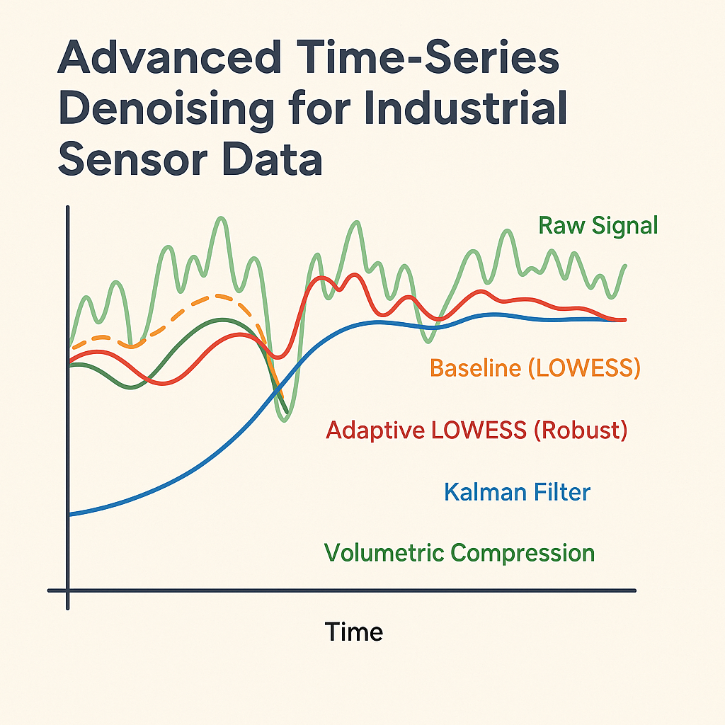
Introduction
Modern industrial systems rely heavily on sensor data — temperature, pressure, oxygen concentration, NOx, flow rates, and countless other process variables. While these measurements are critical for monitoring and control, they often suffer from noise, spikes, and irregular sampling due to:
- Sensor drift or calibration shifts
- Environmental or electrical interference
- Transient system instabilities
- Random measurement noise
Such fluctuations can obscure meaningful trends and mislead predictive models. Therefore, denoising, extracting the “true” signal from noisy observations, becomes an essential pre-processing step in process analytics, predictive maintenance, and anomaly detection.
Traditional methods like moving averages or Gaussian filters are simple but often oversmooth the data or distort peaks. More advanced techniques such as LOWESS (Locally Weighted Scatterplot Smoothing), Adaptive LOWESS, Robust Regression, Volumetric Peak Compression, and Kalman Filtering offer far superior performance, especially in non-stationary, high-variance industrial signals.
This article explores these methods in depth, showing how to combine them effectively for stable, interpretable denoising.
1. LOWESS: The Foundation of Local Regression Smoothing
Concept
LOWESS (Locally Weighted Scatterplot Smoothing) — sometimes called LOESS — is a non-parametric regression technique. Instead of fitting a single global model to the data, LOWESS fits many small local regressions. For each point in the time series:
- A small neighborhood (window) of nearby points is selected.
- Each point in that neighborhood is assigned a weight based on its distance from the target point (closer points have higher weights).
- A simple regression (typically linear) is fit to this local subset.
- The fitted value at the center is the smoothed output.
This process repeats for each point, creating a smooth, adaptive curve that follows the data trend without imposing any specific functional form.
Formula
For a given time t_i, the smoothed value is:

where the weights w(tj,ti) typically follows a tricube kernel:

and di is the distance to the farthest point in the local window.
Intuition
- Small window fraction (
frac) → more responsive to local fluctuations (less smoothing). - Large fraction → more global smoothing (less responsive to fast changes).
This parameter controls the trade-off between trend-following and noise suppression.
Python Example
from statsmodels.nonparametric.smoothers_lowess import lowess

smoothed = lowess(series, np.arange(len(series)), frac=0.1, return_sorted=False)
plt.plot(series, label='Raw Signal', alpha=0.4)
plt.plot(smoothed, label='LOWESS (frac=0.1)', color='orange')
plt.legend()
When to Use
- Suitable for signals with moderate noise and stable variance
- Ideal as a baseline smoother for comparison
- May distort sharp peaks or sudden transitions
2. Adaptive LOWESS: Making the Window Dynamic
Motivation
While standard LOWESS uses a fixed window size (frac), real industrial signals are non-stationary.
In some regions, the signal is stable and slowly varying; in others, it’s noisy or volatile.
Using a single global frac either:
- Oversmooths fast-changing regions
- Leaves too much noise in stable regions.
To overcome this, we introduce Adaptive LOWESS, which adjusts the local window size based on local variance.
Core Idea
We compute a rolling variance of the signal, and dynamically adjust the LOWESS window fraction (frac) as:

Here:
- High variance → smaller window → more responsive smoothing.
- Low variance → larger window → more smoothing.
The square-root damping ensures smooth transitions in window size.
Python Implementation
from statsmodels.nonparametric.smoothers_lowess import lowess

rolling_var = series.rolling(window=20, center=True).var()
var_norm = (rolling_var / rolling_var.quantile(0.9)).clip(0, 1).fillna(0)
adaptive_frac = 0.2 - (0.2 - 0.02) * np.sqrt(var_norm.values)

adaptive_smooth = np.zeros_like(series.values)
x = np.arange(len(series))
for i in range(len(series)):
    f = adaptive_frac[i]
    half_window = max(3, int(f * len(series) / 2))
    start, end = max(0, i-half_window), min(len(series), i+half_window)
    y_fit = lowess(series[start:end], x[start:end], frac=f, it=5, return_sorted=False)
    adaptive_smooth[i] = y_fit[len(y_fit)//2]
Benefits
- Adapts to both stable and volatile regions
- Reduces oversmoothing in fast-changing zones
- Retains trend structure better than fixed LOWESS
Caveats
- Edge behavior can be distorted if window size becomes too small.
- Computationally slower due to pointwise local regression.
To mitigate this, variance can be computed on a downsampled version of the signal first.
3. Robust LOWESS: Handling Outliers Gracefully
Concept
Sometimes, the noise isn’t random, it’s spiky or contains outliers due to sensor faults. Robust LOWESS improves standard LOWESS by iteratively reweighting points based on residuals.
Points far from the local fit (large residuals) receive less weight in the next iteration, reducing their influence.
Example
robust_smooth = lowess(series, np.arange(len(series)), frac=0.1, it=5, return_sorted=False)The it parameter specifies robustness iterations (usually 3–5).
This makes the smoother resistant to sharp outliers or transient spikes.
Benefit
- Suppresses spikes without distorting the underlying pattern
- Essential for industrial datasets with sensor glitches
- Works beautifully when combined with Adaptive LOWESS
4. Adaptive Robust LOWESS (Hybrid Approach)
The Adaptive Robust LOWESS combines the ideas from above:
- Adaptive variance-based windowing
- Robust reweighting for outliers
This hybrid approach intelligently smooths highly non-stationary signals — such as kiln oxygen levels or combustion chamber NOx — without losing important transients.
Example: Adaptive Robust LOWESS Code
var_window, clip_ratio = 20, 90
min_frac, max_frac = 0.02, 0.2
robust_it = 5

rolling_var = series.rolling(window=var_window, center=True, min_periods=3).var()
var_norm = (rolling_var / rolling_var.quantile(clip_ratio/100)).clip(0,1).fillna(0)
adaptive_frac = max_frac - (max_frac - min_frac) * np.sqrt(var_norm.values)

adaptive_frac = np.clip(adaptive_frac, min_frac, max_frac)
adaptive_smooth = np.zeros_like(series.values)

x = np.arange(len(series))
for i in range(len(series)):
    f = adaptive_frac[i]
    half_window = max(3, int(f * len(series) / 2))
    start, end = max(0, i-half_window), min(len(series), i+half_window)
    y_local = series.iloc[start:end]
    if len(y_local) > 6:
        y_fit = lowess(y_local, x[start:end], frac=max(0.05,f), it=robust_it, return_sorted=False)
        adaptive_smooth[i] = y_fit[len(y_fit)//2]
    else:
        adaptive_smooth[i] = series.iloc[i]
5. Volumetric Regression: Selective Peak Compression
Problem
Sometimes, even after denoising, sharp peaks remain — not noise per se, but physically unrealistic excursions that disrupt downstream modeling. We want to reduce their volume, not remove them entirely.
That’s where Volumetric Regression (or Peak Compression) comes in.
Concept
- Use LOWESS to get a baseline trend.
- Compute deviation from baseline.
- Use robust IQR-based thresholds to detect local peaks and dips.
- Compress only the amplitude of these deviations while leaving the rest untouched.
Example Code
baseline = lowess(series, np.arange(len(series)), frac=0.07, return_sorted=False)
deviation = series - baseline

q1 = deviation.rolling(15, min_periods=1).quantile(0.25)
q3 = deviation.rolling(15, min_periods=1).quantile(0.75)
iqr = q3 - q1

upper, lower = q3 + 0.5*iqr, q1 - 0.5*iqr
peak_mask = (deviation > upper) | (deviation < lower)

compression_strength = 0.4  # between 0 (flatten) and 1 (no change)
compressed = series.copy()
compressed[peak_mask] = baseline[peak_mask] + compression_strength * deviation[peak_mask]
Use Case
- Reduces false alarms in anomaly detection systems.
- Keeps trend integrity while damping spike amplitude.
- Useful in kiln O₂, NOx, or temperature data.
6. Kalman Filtering: Model-Based Denoising
Concept
While LOWESS and its variants are data-driven, the Kalman Filter is model-based. It assumes a dynamic system governed by equations of motion and recursively estimates the system’s state given noisy observations.

The Kalman Filter updates its estimate of xt by balancing model prediction and measurement noise.
Simplified 1D Implementation
from pykalman import KalmanFilter

kf = KalmanFilter(initial_state_mean=series.iloc[0],
                  n_dim_obs=1, n_dim_state=1,
                  transition_matrices=[1],
                  observation_matrices=[1],
                  transition_covariance=0.1,
                  observation_covariance=1.0)
Tuning
- Increase
transition_covariance→ more responsive (follows signal). - Increase
observation_covariance→ smoother (trusts model more than data).
Combining Kalman with LOWESS
You can use the Adaptive LOWESS output as the observation model for Kalman Filtering, achieving:
- Adaptive trend tracking (from LOWESS)
- Statistical noise control (from Kalman)
This hybrid is particularly effective for control loops and emission monitoring systems.
Comparative Summary

8. Practical
Tuning Workflow
- Start with baseline LOWESS to understand trend.
- Add robustness (
it > 3) to handle spikes. - Incorporate adaptive variance windowing if signal volatility changes.
- Use volumetric compression only if peaks dominate behavior.
- Layer Kalman Filtering for state estimation or predictive models.
9. Example Visualization Workflow
Combine all together:
plt.figure(figsize=(18, 6))
plt.plot(series, label="Raw Signal", alpha=0.4, color="green")
plt.plot(baseline, label="Baseline (LOESS)", color="orange")
plt.plot(adaptive_smooth, label="Adaptive LOWESS (Robust)", color="red", linewidth=2)
plt.plot(smoothed, label="Kalman Filter", color="blue", linewidth=1.8)
plt.legend()
plt.title("Comparative Denoising – Industrial Sensor Signal")
plt.xlabel("Time")
plt.ylabel("Measurement Value")
plt.grid(True)
plt.tight_layout()
plt.show()
🚀 10. Key Takeaways
- LOWESS is an excellent general-purpose smoother for capturing slow trends.
- Robust LOWESS handles outliers effectively.
- Adaptive LOWESS dynamically tunes smoothing for changing variance.
- Volumetric Regression selectively compresses peaks, preserving realism.
- Kalman Filters combine physical intuition and statistical inference.
For industrial process data — such as kiln O₂, NOx emissions, furnace pressures, or cooling water flow — these hybrid techniques can dramatically improve signal clarity, fault detection, and predictive stability.
Final Thoughts
In the world of process analytics, no single filter is perfect. The best denoising pipelines blend statistical adaptivity, robustness, and physical interpretability.
- Use Adaptive LOWESS for real-time trend monitoring.
- Use Volumetric Compression to smooth occasional spikes.
- Layer Kalman Filtering when a system model is known or estimated.
By combining these, you move from simply “cleaning data” to intelligently reconstructing the underlying process behavior — a critical capability in data-driven manufacturing and advanced process control.
메타데이터
- post_id
- a1ba0879e79d
- slug
- advanced-time-series-denoising-techniques-for-industrial-sensor-data-a1ba0879e79d
- url
- https://medium.com/@athi.9307/advanced-time-series-denoising-techniques-for-industrial-sensor-data-a1ba0879e79d
- canonical_url
- https://medium.com/@athi.9307/advanced-time-series-denoising-techniques-for-industrial-sensor-data-a1ba0879e79d
- author_url
- https://medium.com/@athi.9307
- status
- ok
- fetched_at
- 2026-08-03 00:21:16