Doppler Effect & Redshifts In Astronomy

The Doppler effect, named after Austrian mathematician Christian Doppler, is often depicted with the sirens of a car coming from far away, passing by, and eventually moving away. Upon imagining this situation, we observe that the sound frequency varies depending on where the car is relative to us.

It is this change in frequency as an object moves and emits waves, applying to all types of waves, that is known as the Doppler effect. We will proceed by building a progressive framework of the Doppler effect to understand its applications in advanced astronomy.

At the same time, we will study the different types of redshift as well as how it links to the Doppler effect.

Physical Interpretation Of The Doppler Effect

Let’s imagine the following situation, where a car is moving towards an observer at the speed v. Meanwhile, the car is sending waves propagating at speed c. We place ourselves in the reference frame of air, and will denote the observer’s speed u.

We will state that v < 0 if the car is going the other way, and will apply the same principle to the observer, thus u < 0. We come to:

Sound waves Doppler effect postulated situation

If we decide to think about the waves as tiny marbles, we can find the frequency at which an observer receives them. The frequency at which a marble is emitted will be denoted fe, and fr will refer to the frequency at which it was received.

At t = 0, the car has a certain position, but at t = T, the car has travelled a certain distance d = vT and has a different position. If the car emits a marble at t = 0, the following situation at t = T would occur:

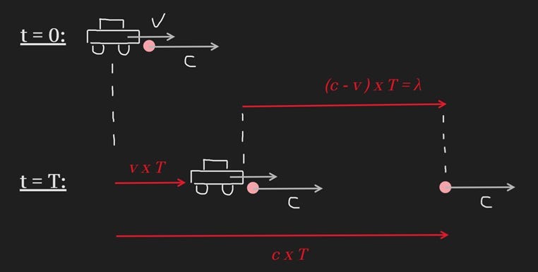
System’s motion over a period of time T

Now let us imagine that the car emits another marble at t = T, then we are looking for the distance between the two marbles at time T. We can work out that this distance is equal to cT — vT or T(c-v) = λ. This is the wavelength of the sound wave in the reference frame of air.

We will now propose a different origin of time at which the observer receives the marble, such that:

System’s motion over a period of time T’ from a different origin of time

Where the observer receives the marble at time t = T’, while moving at speed u. We deduce that cT’ = λ + uT’, and arrive at (c-u)T’ = λ. Using this expression, we come to T(c-v) = (c-u)T’ and to:

As the frequency is inversely proportional to the period.

Finally, we can express:

From this expression, we understand that if the observer remains stationary, fr = fe c/(c-v) = fe 1/(1-(v/c)) and that if the car is coming towards the observer, 1/(1-(v/c)) > 1 meaning that fr > fe, leading to a more high-pitched sound. Conversely, if the car is getting away, v < 0, c — v > c and 1/(1-(v/c)) < 1, the sound is more low-pitched.

Physically, this shows how the received waves depend on the speed of the emitting object.

Doppler Effect Of Electromagnetic Waves

Now, the Doppler effect is well known through the example we have used, that of a car whose sound’s frequency is modified according to where it is relative to the observer; but the key insight behind the Doppler effect is that it applies to all types of waves.

This includes electromagnetic waves, commonly referred to as light. Now this is interesting, light does not produce sound, so how could the Doppler effect affect it?

In fact, the frequency of electromagnetic waves is also altered by this effect, but this has a different consequence than modifying the pitch.

Let us first imagine a similar situation to that presented previously. This time there is no medium: light does not require one to propagate, which is a key difference from the sound‑wave case.

Special Relativity postulates that the speed of light c is the same for all observers in all inertial reference frames. This signifies that we do not require to take into account the movement of an observer, we can choose a reference frame in which the observer remains stationary to simplify the situation, and find the same result.

Drawing a 2D spacetime diagram, we obtain the following state:

Spacetime diagram of the relativistic postulated situation

Now, if we write the observer’s trajectory vector, that of the car, and the wavevector for light, we can express respectively as:

Because the observer is only moving in the time direction, since the movement in space is determined by the speed of the car. And because light moves at speed c.

Labelling fe and fr the frequencies respectively emitted and received, we can project using a dot product, the wavevector (1 c) on (1 0) which is defined only in the time direction. Thus, we are counting the number of oscillations during one unit of time through this projection, which exactly corresponds to the definition of frequency. We obtain:

Now from its reference frame, the car is stationary. This modifies its time axis to be that oriented by the car’s vector. We work out that:

Using Minkowski’s metric, which describes flat spacetime in Special Relativity, we adapt the expressions of the dot product and norm, and calculate that:

Replacing in the formula, we obtain fr = c.

Note that the units are not corresponding as fr is a frequency and c a velocity. This is because we chose vectors arbitrarily and thus has no physical meaning. Rather, we will interpret fr /fe.

We find:

So;

At last, we obtain the formula for the relativistic Doppler effect.

Immediately, we see that this formulation differs from that of a sound wave. In fact, the physical interpretation is also contrasting, as for a sound wave the pitch is modified, but for light, the increase of wavelength, proportional to that of frequency, induces color variations.

Light thus appears in a different color than the color it was emitted with. This is more commonly known as redshift and blueshift.

Doppler Redshift

Therefore, redshift is one of the central application of the Doppler effect in astronomy. When a star or galaxy emits particles of light (photons), we observe a certain spectrum of light, called an absorption spectrum. Absorption spectra scan across the full visible range of the electromagnetic spectrum (400 nm to around 700 nm).

Now, at some specific wavelengths, we observe not the color we expect but a dark band. This means we have not received photons carrying this specific wavelength, meaning that between us and the source of the photon emission lie atoms which absorbed that specific wavelength.

Thus, each element has a characteristic absorption‑line spectrum determined by its constituent atoms. But now, if the emission source of the photon is moving, the frequency of the photon changes and so does the wavelength.

Thereby, even though the absorption lines have not been modified, the absorption spectrum is shifted due to the change in wavelength. The change in wavelength also induces blueshift if the source moves toward us (the wavelength decreases), and redshift if it moves away from us (the wavelength increases).

Now, from this shift and because we know the rest wavelengths λ0 at which atoms absorb photons, we are able to work out the fractional shift from the observed wavelength λ.

We find that:

For most stars and galaxies at non-relativistic speeds, the Doppler relation can be approximated as:

with vr the radial velocity.

Relativistically, astronomers use the formula we previously derived but with wavelengths instead of frequencies, as they are inversely proportional such that:

And define redshift z as:

(while keeping the sign convention introduced earlier: v < 0 for a receding source and v > 0 for an approaching source)

Cosmological Redshift & Lookback time

The Doppler effect is not the only source of the observed redshift. Observations reveal that more than one effect of redshift is often present, leading astronomers to talk about effective redshift as the sum of all redshift sources applied to an object.

As the universe is expanding, so is spacetime. Because of this, we observe cosmological redshift as the electromagnetic waves inside the fabric are stretched along with it.

Now, stretching a wave merely comes down to increasing its wavelength, explaining the tendency of visible light to tend towards infrared, and even further if emitted near the beginning of the universe. For instance, the light produced by the Cosmic Microwave Background at redshift z = 1,100 (380,000 years after the Big Bang) has stretched to the microwave domain.

Cosmologists use cosmological redshift to determine distances through Hubble’s Law V = H0d, and to work out the age of structures, or at least from which epoch they originate.

In 1922, upon applying the equations of General Relativity to the universe itself, Alexander Friedmann worked out two equations modeling the expansion of the universe. To describe it, he used the scale factor a(t).

Therefore, cosmological redshift can also be interpreted as the ratio between the value of the scale factor at the moment a wave is observed over its value when the wave was emitted. It follows that:

By convention, using aobserved = 1, one can define the size of the universe at the time of wave emission while knowing how redshifted that wave is. Merely, we find that:

On large scales, typically hundreds of megaparsecs (1 pc = 3.26 light-years) and more, cosmological redshift dominates over local motions, and thus helps cosmologists to map the large scale structure of the universe.

Now, cosmologists use cosmological redshift to calculate lookback time, the time that elapsed since the light from a distant object was emitted. This is directly related to how long light has been traveling towards Earth.

Cosmic age at redshift z, is how old the universe was when the light was emitted. This equals the present age of the universe minus the lookback time, and is given by:

tL(z): Lookback time

And with H(z) the Hubble parameter as a function of redshift z, with Ωm the matter density, ΩΛ the dark energy density, and H0 the Hubble constant, such that:

The exact integral cannot be solved analytically for the general case but then excellent analytic approximation accurate to better than 0.1% for all redshifts is:

With the Hubble time in billions of years:

Using Λ-CDM cosmology parameters (H0 = 70 km/s/Mpc, Ωm = 0.3), values for lookback times from measured redshifts can be determined.

Gravitational Redshift

Another type of redshift to consider is gravitational redshift. This phenomenon occurs when an electromagnetic wave climbs out of a gravitational potential well in General Relativity.

As time dilation is stronger in a gravitational field, light emitted at a lower gravitational potential, appears to possess a lower frequency (in turn a longer wavelength as c = λf) to an observer located at a higher potential.

Equivalently, this effect can be thought of as the photon losing energy (along the relation E = hν, with ν the frequency of the wave, and h Planck’s constant), during its escape of the gravitational well.

The energy required to leave the well affects the wave frequency, effectively reducing it (increasing wavelength), and translating into redshift. We will build an example using this logic.

Let us imagine two observers around a black hole, which will be described using the Schwarzschild metric, and will be considered to possess a radius rs (Schwarzschild’s radius):

We will consider that the two observers remain stationary around the black hole and will denote them as A and B. Now, A sends a light ray with a certain spacetime wavevector, which gets deviated by the black hole before arriving to B with another wavevector, such that:

Black hole’s gravitational redshift postulated situation

Note that both observers also have a spacetime vector, which are only directed in the time direction as both observers remain stationary in the space dimension.

We know that:

And:

We will note rA and rB the altitudes of both observers. Using the coordinates (t, r, ϕ) we have:

Since dt2=1, dr = 0 and dϕ = 0, we get:

Now, to find the geodesic (shortest path) that links A to B, we need to work out a relation between the wavevectors. We have:

As we are only considering the time dimension because both space dimensions will not affect the calculation since the metric is diagonalized and that the spacetime vectors are only expressed in the time dimension.

To find a relation between the wavectors, we note that Schwarzschild’s metric is invariant over time, thus, according to Noether’s theorem, there is a symmetry in the metric and thereby, a conservation along the geodesic followed by the light ray. In particular, the conserved quantity is the derivative of ds2 over dt such that:

Because this quantity is conserved, if we replace dt with ωA or ωB, it will remain the same value — we find the following equation:

Replacing to work out the frequencies, we obtain:

And from the derived relations, we deduce that:

This is because the spacetime vectorsare temporal and that the temporal vector represents a symmetry of the metric, since the metric does not over time.

Noether’s theorem implies the conservation of:

More precisely, we say that the spacetime vectors represent a Killing vector field (a symmetry of spacetime so that the wavevector with the Killing vector, here the spacetime vector associated, must remain constant).

Finally, we find that:

This is the final equation for the effect of gravitational redshift in the Schwarzschild metric for two stationary observers exchanging a light ray.

We see that if B is far from the black hole:

So B receives a weaker frequency, thus a redshift frequency, and sees A moving slower due to gravitational time dilation.

Otherwise, if A receives the wave:

The wave is blueshifted and A sees B moving faster.

Blueshift

These effects can also in certain cases create blueshifted objects. Merely, blueshift occurs when the wavelengths decreases; and redshift z exhibits a negative value. The existence of blueshifted objects reveals that at sufficiently small scales, gravitational attraction overwhelms the expansion of the universe.

In fact, Hubble’s expansion operates primarily on scales greater than 5 Mpc, as within this distance attraction dominates.

The most prominent blueshifted objects are galaxies within our local group (grouping of galaxies). The Andromeda galaxy (M31) exhibits a blueshift of z = -0.00042 indicating an approach velocity of around 100 to 125 km/s.

Another example is the Virgo cluster (M90) which recedes as a whole from us, however, M90 moves toward us at sufficient velocity to exhibit a blueshift. Astronomers attribute this to the cluster’s enormous gravitational field, accelerating member galaxies to extreme velocities, sending some toward Earth while others recede.

Now, because at close scale gravitational fields overcome the expansion of the universe, not only galaxies but also stars possess blueshift, even if weaker. For instance, Barnard’s star exhibits blueshift, detectable through high resolution spectroscopy of well-defined hydrogen absorption lines.

Radial Velocity Applications

Now, radial velocity vr is the line-of-sight component of an object’s velocity, in other words, how fast it is moving towards or away from us. It is defined as positive for redshift and negative for blueshift.

In practice, astronomers measure radial velocity by comparing the wavelengths of spectral lines obtained from observations, to their laboratory rest values. This amounts to work with the Doppler relation approximated for non-relativistic speeds, such that:

Modern spectrographs (instruments spreading incoming radiation into its component wavelengths and recording the resulting spectra for analysis) reach precisions of around 1 to 10 km/s for large surveys, such as ESA’s Gaia mission. Other missions go up to 1 m/s for specialized exoplanet-hunting instruments.

This precision factor allows astronomers to reconstruct the 3D velocities of stars across the sky.

Indeed, if we know the distance to the star, through Cepheid variables or Hubble’s Law (find more about it in my article: Measuring the universe: Cosmic distances and Stellar properties — How did man uncover as much with as little?), plus its motion relative to our line-of-sight, we can work out the other velocity components to map three-dimensional motion.

This approach can also be applied to interstellar gas to constrain the mass distribution (including dark matter) and the interplay between gas flows and star formation.

In unresolved binary systems, the periodic changes in the radial velocity of one or both components reveal orbital motion. By fitting the radial-velocity curves, astronomers derive orbital periods, eccentricities, and mass functions which in turn, solve for accurate stellar masses if inclination constraints are known.

This is the study of spectroscopic binaries, binary star systems whose components are too close together to be resolved as separate objects using a telescope.

Moreover, detecting radial velocity variations over multiple Gaia epochs also flags multiple star systems statistically in huge stellar samples, even when the orbit is not fully characterized.

Now, Radial velocity is most often referred to as a method to discover exoplanets. According to IRAP’s studies around 1,100 exoplanets have been detected using this method out of more than 6,000 exoplanets known, as of March 2026.

The radial velocity detection method is founded on the fact that a planet’s gravity causes its star to wobble slightly in its orbit, allowing astronomers to observe a periodic shift in the light spectra, due to the Doppler effect.

This method reveals the minimum planet mass, as large wobbles induce a heavier planet, as well as the orbital period and shape (circular or elliptical mainly). Overall, this method works best for massive planets; small planets produce tiny stellar wobbles that require much higher precision to detect.

Advanced Application: Relativistic Beaming

A more advanced application of the Doppler effect is found in relativistic beaming (also Doppler beaming), the combination of aberration, Doppler shift, and time dilation, that makes radiation from a source moving at relativistic speed appear strongly concentrated and amplified in the direction of motion, while being suppressed in the opposite direction.

Concretely, at relativistic speeds, light rays contract and focus, amplifying brightness in the direction of motion. This is called the aberration of light, but remains a fictitious effect in the sense that only the observer moving at a relativistic speed perceives it.

This is somewhat analogous to driving a car very fast when it is raining. Indeed, the rain seems to hit the windshield with a certain angle whereas rain is actually falling vertically.

Extrapolating this situation will increase the angle, focusing more and more the light rays, thus amplifying brightness in the direction of motion while suppressing it in the opposite direction..

If we couple this effect with Doppler’s and time dilation, which occurs significantly enough in extreme gravitational fields or at advanced relativistic speeds, we obtain relativistic beaming.

Thus, relativistic beaming is central to interpreting the extreme brightness, variability, and jet asymmetries of quasars (extremely luminous active galactic nuclei), blazars (type of quasar whose astrophysical jet is pointed almost directly at Earth), and accreting (or in possession of an accretion disk) black holes.

Artist’s view of a supermassive black hole accreting and releasing an astrophysical jet — MIT

These astronomical objects are so powerful, they produce relativistic plasma jets along their magnetic axis. From the plasma’s rest frame, the jet can be modeled as radiating roughly isotopically (similarly in all directions).

Now, in the observer’s frame, Lorentz transformation (coordinate-conversion rules between two inertial frames moving at constant relative velocity in Special Relativity) of photons causes aberration of light due to relativistic speeds.

Taking into account Doppler shift and time dilation, both correlated to relativistic speeds, we find that most of the apparent power is emitted into a narrow cone of opening angle ~ 1/Γ around the direction of motion. Note that in reality, other redshift effects like cosmological and gravitational are to take into account.

Here, Γ represents the Lorentz factor γ:

Specifically in the context of relativistic astrophysics, and more precisely to denote the bulk motion of photons (average velocity) in percentage of c.

Interestingly, we notice that the closer Γ is from c, the narrower the opening angle, and thus the stronger the effect. A raw calculation at v = 0.99c (typically the lower bracket of speed for such jets), gives γ ~ 7.09, and therefore, an opening angle of around 8.1°.

Because of this, plasma moving toward us appears much brighter than the same plasma at rest, while plasma moving away appears dramatically fainter; this is why many AGN show a bright one‑sided jet while the counter‑jet is weak or invisible.

Thereby, the Doppler effect is central in astronomy, allowing astronomers to discover exoplanets, determine their properties as well as that of stars and galaxies, but also to comprehend the motion and effects of the powerful jets produced by AGNs.

Christian Doppler’s work remains fundamental on Earth and across the universe, shaping our understanding of motion, light, and the dynamic nature of reality itself.

Julien CEREZO

Space engineering student, future PhD student in Astrophysics

Online writer and editor, conference speaker, popularizer

Credits: Mathematical derivations, Alessandro Roussel — Scienceclic