Beyond Correlation: How We Used Causal Inference (FCI) to Break the Feedback Loop in Our ML Models

Why your non-linear models are still learning fake correlations, what “Causal Boundaries” actually mean for your data, and a practical roadmap to fix it.

Introduction: The Confession of a Data Scientist

Let’s be honest, we’ve all been there. You build a sophisticated, highly non-linear model — perhaps using XGBoost or a deep neural network. You carefully split your dataset, run cross-validation, and achieve phenomenal validation metrics (Accuracy / ROC-AUC). The model goes into production with great pride, the charts look amazing for the first few weeks, and then… a month or two later, performance begins to degrade at an alarming rate, or the model starts making bizarre product decisions.

The automatic response in the industry is often: “Ah, we have Data Drift, let’s just retrain the model on last week’s data.” So, you set up a pipeline for Daily Re-training. But the real problem is much deeper than that.

When your model operates within a live system, it changes reality. Users see its recommendations and act on them. This means the data generated tomorrow is a direct consequence of the model you trained yesterday. Your model becomes trapped in a dangerous Feedback Loop. It stops learning what actually drives user behavior, and instead, it starts learning the spurious correlations that the system itself created.

To break this loop, we must take off our classical correlation glasses and put on a new pair: Causal Inference. In this article, we will dive into two advanced concepts that are changing the game in the industry: the FCI algorithm and the concept of Causal Boundaries.

Part 1: The Invisible Enemy — Latent Confounders

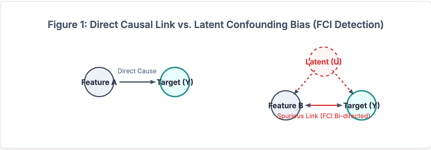
In basic statistics courses, we are taught about “confounders” — variables that simultaneously affect both the feature (the apparent cause) and the target (the effect). The classic example is the correlation between ice cream sales and shark attacks; the confounding variable is “warm summer weather.”

If the confounding variable is measured and exists in our data (Observed), it’s easy to adjust for it using methods like Regression Adjustment or Propensity Score Matching. However, in the real world of tech and product data, the most dangerous variables are those that we cannot measure. These are Latent Confounders.

Imagine we are developing a model that calculates the “attractiveness” of an item or user in a marketplace system. Suppose there is a hidden factor like “high user self-awareness” or an “underground cultural trend on social media.” This component isn’t stored in any SQL table, but it significantly affects both the features the user generates and their conversion potential. A standard ML model will take the visible features and over-weight them simply because they correlate with the hidden factor, leading to catastrophic prediction failures the moment that latent trend shifts.

Part 2: Meet FCI (Fast Causal Inference)

To discover causal relationships from observational data, there is a family of algorithms called Causal Discovery. The most famous among them is the PC Algorithm (named after Peter Spirtes and Clark Glymour). However, the PC algorithm makes a bold and often unrealistic assumption: that there are no latent confounders (Causal Sufficiency).

This is where the FCI (Fast Causal Inference) algorithm comes in. Developed by Spirtes, Glymour, and Scheines, FCI’s unique and powerful feature is its ability to handle messy reality: it does not assume the absence of latent confounders, and it can also account for Selection Bias.

Instead of generating a standard causal graph (DAG), FCI produces a mathematical structure called a PAG (Partial Ancestral Graph). In this graph, different types of edge-ends can tell us: “There is a correlation between Feature A and Feature B, but I mathematically detect that there is a hidden factor misleading you (represented as a bi-directed arrow A ↔ B).” FCI achieves this through a series of Conditional Independence Tests that isolate information pathways.

Part 3: Cracking “Causal Boundaries” & the Markov Blanket

So what exactly is a “Causal Boundary” in data analysis? A great way to define it mathematically is through the concept of the Markov Blanket.

For a specific target variable ($Y$), its Markov Blanket consists of:

1. Its direct parents (variables that directly cause $Y$).
2. Its direct children (variables that $Y$ directly causes).
3. Its children’s other parents (variables that share a child with $Y$).

The Markov Boundary Rule: If we know and perfectly measure all variables within the Markov Blanket of $Y$, all other variables in the universe become completely irrelevant (conditionally independent) for predicting $Y$. The Markov Blanket is the absolute causal boundary of information.

The severe problem with modern ML models is that they bleed past the Markov Blanket. Since a model like XGBoost only looks for ways to minimize loss in the training set, it will happily exploit features far outside the causal boundary, as long as they have a temporary statistical correlation with the target. Once the environment shifts or the model itself alters the market dynamics, these spurious links collapse, rendering the model useless.

The fix for this is Causal Regularization: we use an algorithm like FCI to identify the true Markov Blanket and strictly penalize or entirely drop features that attempt to cross this causal boundary without a genuine causal justification.

Part 4: From Theory to Production (A Practical Roadmap)

When presenting these ideas to management, the biggest hurdle is always ROI. Managers will rightly say: “This sounds amazing theoretically, but how much will it actually improve our KPIs? Is it worth weeks of engineering effort?”

The secret is not to build a complex production infrastructure all at once, but to conduct focused Offline Evaluation to prove statistical impact in minimum time. Here is the practical roadmap we utilized:

1. Estimating Causal Regularization Impact Offline

Instead of altering the live model, isolate a chunk of historical data (e.g., from a previous quarter). Train two models side-by-side: your original non-linear model, and a “bounded” model where you manually drop or heavily penalize all features that the FCI algorithm flagged as outside the Markov Blanket. Then, test both models on future data (Out-of-sample / Out-of-time). If the causally regularized model maintains higher and more stable accuracy over time, you have your first numerical proof of the causal boundary’s value.

2. Breaking Feedback Loops via Inverse Probability Weighting (IPW)

Our models tend to train on biased data because they learn from their own past choices. The ideal long-term fix is an active randomized exploration mechanism (like Multi-armed Bandits), but that requires significant engineering overhead.

As a rapid offline workaround, you can use a statistical technique called Inverse Probability Weighting (IPW). This method allows us to retroactively “de-bias” historical model decisions. By giving higher weight to rare observations that the model previously ignored, we simulate a clean, unbiased data collection process. Comparing the offline loss of an IPW-adjusted model against a standard model will give management an exact estimate of the expected performance lift.

Conclusion: The Causal Revolution in Data Science

The field of Data Science is undergoing a dramatic paradigm shift. Leading tech companies are realizing that a high validation accuracy score is a dangerous illusion if the model operates in a dynamic environment and continuously alters its own inputs.

Moving to non-linear architectures or setting up daily retraining schedules are valuable steps, but they do not solve the root issues of spurious correlations and systemic feedback loops. The next time you analyze your model’s feature importance, stop and don’t just ask: “How much does this feature contribute to the prediction?” Ask yourself: “Does this feature live inside the Causal Boundary, or is it just surfing a temporary wave of correlation?”