From Scalar to Spectral: How One Simple Equation Keeps Its Power in Higher Dimensions

How One Simple Equation Keeps Its Power in Higher Dimensions

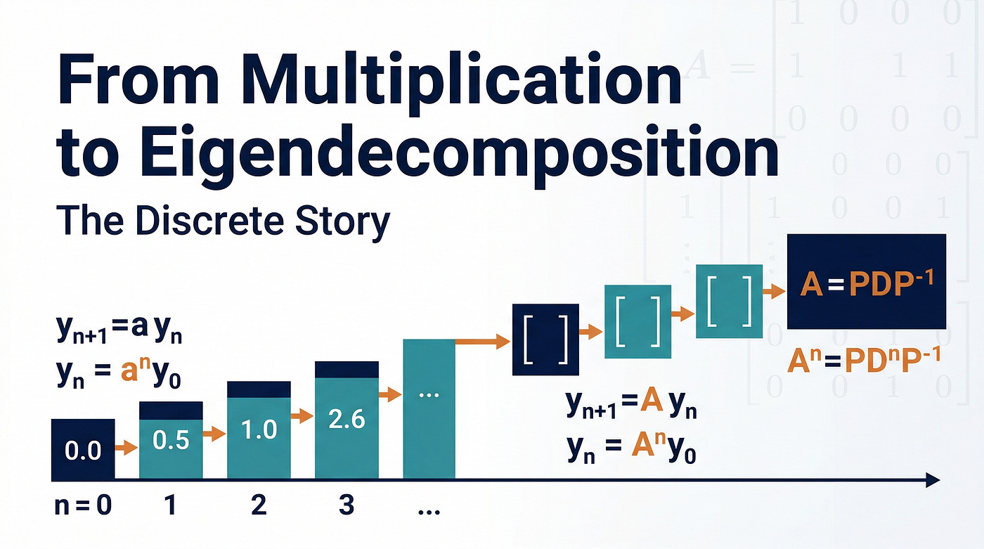
The Seed

All of mathematics occasionally offers a moment where a single, almost trivially simple idea contains the DNA of something vast. The ordinary differential equation

dy/dt ​= ay

is one such idea. It says: the rate at which something changes is proportional to how much of it there is. Populations grow this way. Radioactive atoms decay this way. Bank accounts compound this way. The solution is immediate and elegant:

y(t) = y₀​ eᵃᵗ,

where y₀​ is the initial state and a is the rate. The exponential function eat is the bridge between the present and the future. For a single quantity evolving at a single rate, this is the complete story.

But the world rarely consists of a single quantity evolving in isolation.

The Leap

Suppose instead of one variable we have n of them, coupled together. The temperature at one point in a rod depends on neighboring points. The concentration of one chemical species in a reaction depends on the concentrations of others. The state of an economy depends on the interplay of many sectors.

We collect these variables into a vector y(t) and their couplings into a matrix A, and the system becomes

dy​/dt = Ay.

By sheer analogy with the scalar case, we are tempted to write

y(t) = eᴬᵗy₀​,

and this turns out to be correct. But now we face a question that did not exist before:

What does it mean to exponentiate a matrix?

The Definition and Its Burden

The matrix exponential is defined by the same Taylor series that defines the scalar exponential:

eᴬ**ᵗ** = I + At + A²t²/2! ​+ A³t³​/3! + ⋯

This is mathematically precise. It converges for any square matrix A. It is also, in practice, a burden.

Because hidden inside that innocent-looking series is the true difficulty:

The exponential is made of powers. To compute or understand eᴬ**ᵗ**, you must confront A²,A³,A⁴,…

And matrix powers are exactly where the “mixing” lives. Each multiplication entangles entries further; structure that was visible in A gets scrambled in A², worse in A³, and so on.

Figure 1. Repeated multiplication makes the matrix “mix” more and more — exactly the pain point inside the exponential series.

So there is a gap — the moment where the simplicity of y =y₀​ eᵃᵗ seems to abandon us as we step into higher dimensions. The definition tells us the object exists. It doesn’t yet tell us how to compute it without drowning in powers.

The Diagonal Exception

There is, however, one class of matrices where everything remains simple. If A happens to be a diagonal matrix

then its powers are trivial. Each diagonal entry simply raises to the kth power independently:

And the Taylor series collapses term by term:

Each entry on the diagonal is a scalar exponential — exactly the function we started with. The matrix exponential of a diagonal matrix is nothing more than n independent copies of the scalar exponential.

Figure 2. When the matrix is diagonal, powers stay simple — so the exponential becomes “n scalar stories in parallel.”

So the question becomes sharply focused:

Can we reduce a general matrix to this diagonal paradise — without changing the dynamics, only our point of view?

The Bridge (Seen Through Powers)

Suppose the matrix A possesses n linearly independent eigenvectors v₁​,…,vₙ​ with corresponding eigenvalues λ₁​,…,λₙ​, satisfying

*Avᵢ = λ*ᵢ​ vᵢ​.

Each eigenvector defines a direction in which A acts by pure scaling — no mixing, just multiplication by a number. If we assemble these eigenvectors as columns of a matrix P and the eigenvalues into a diagonal matrix D, we obtain the factorization

A = PDP⁻¹.

This is the moment the story quietly turns: not because a new symbol has appeared, but because a new mechanism has arrived.

The mechanism is cancellation

Watch what happens to powers:

A² = (PDP⁻¹)(PDP⁻¹) = PD(P⁻¹P​​)DP⁻¹= PD²P⁻¹.

Do it again:

A³ = A²A = (PD²P⁻¹)(PDP⁻¹) = PD²(P⁻¹P​​)DP^−1=PD³P⁻¹.

And now the pattern is unavoidable:

Aᵏ = P Dᵏ P⁻¹ for all integers k ≥ 1.​

The inner products P⁻¹P collapse to the identity at every step, and only the diagonal matrix accumulates powers — which, as we established, is trivial.

Figure 3. The “secret engine”: repeated P⁻¹P=I cancellations turn hard powers Aᵏ into easy powers Dᵏ.

If the scalar story was powerful because powers were easy, then the spectral story is powerful because it rebuilds that same ease: not by changing the system, but by choosing coordinates where repeated multiplication has a simple core.

The Payoff

Now return to the Taylor series definition. The exponential demands powers:

eᴬᵗ= I + At + A²2t²​/2!​ + A³​t³​​/3! + ⋯

But we have just learned that every power has the form Aᵏ = P Dᵏ P⁻¹. Substitute that into the series: every term carries a P on the left and a P⁻¹ on the right, so they factor out cleanly:

eᴬ**ᵗ** = P(I + Dt + D²​2t²​​/2! + ⋯)P⁻¹ = P eᴰᵗ P⁻¹.

And since D is diagonal, eᴰᵗ is just scalar exponentials on the diagonal.

So the full solution becomes

y(t) = P eᴰᵗ P⁻¹ y₀​.

If we define z₀​ = P⁻¹ y₀— the initial condition expressed in the eigenvector basis — then the solution reads like a superposition of independent scalar stories:

y(t) = z1,0​ e^λ1​*t *v1 ​+ z2,0 ​e^λ2​t v2​ + ⋯ + zn,0 ​e^λn​t v*n*​.

Each mode is, once again, the original scalar solution y = y₀​ eᵃᵗ — now carrying a direction as well as a magnitude.

Figure 4. Change basis → evolve independently in the diagonal core → change back. The scalar simplicity is recovered “in the middle.”

The Circle

The story begins with a scalar equation and its exponential solution. It ventures into the matrix world, where the exponential becomes opaque because it is built from powers A²​,A³​,…. It discovers that diagonal matrices preserve the simplicity of the scalar case. And it finds a bridge: a way to write A so that powers stop being a swamp and become a sidewalk.

Underneath all the terminology, the nature of the spectral viewpoint in this story is simple:

• eigenvectors are directions that don’t mix,
• eigenvalues are the rates along those directions,
• and the reason the whole construction is useful is that it makes powers easy:

(PDP⁻¹)ᵏ= P Dᵏ P⁻¹

That identity is the hinge on which the exponential swings.

Figure 5. The geometry behind “no mixing”: along special directions, the transformation behaves like pure scaling.

It all begins, and ends, with y′=ay — because the exponential story never really changed. We only learned how to tell it in the coordinates where multiplication stays simple.