EVRP Using Python : A Practical Guide to Optimization Model Implementation

Building a Complete Pipeline with Data Generation, Optimization, Validation, and Visualization

Electric vehicles (EVs) are rapidly transforming modern logistics and transportation systems. Unlike traditional delivery vehicles, however, EVs introduce an additional operational constraint: limited battery capacity.

The classical Vehicle Routing Problem (VRP) focuses on determining the shortest or lowest-cost routes for delivering goods to customers. Traditional VRP formulations generally assume that vehicles can travel indefinitely as long as routes are optimized efficiently. The Electric Vehicle Routing Problem (EVRP) fundamentally changes this assumption because route feasibility now depends on energy availability.

As a result, EVRP introduces several additional real-world considerations, including:

• Limited battery capacity
• Energy consumption based on travel distance
• Charging station selection decisions
• Recharging penalties and delays
• Operational trade-offs between travel efficiency and charging behavior

These additional constraints make EVRP significantly more complex and substantially more realistic than classical routing problems.

In the previous article, we discussed the mathematical formulation of the EVRP optimization model. In this article, we implement the EVRP model using Pyomo. However, the objective of this article is not just to solve a single fixed instance, but to create a framework capable of generating and solving multiple routing scenarios.

[embed]From Shortest Paths to Energy-Efficient Routes: Extending TSP to EV Routing A step-by-step MILP formulation with battery constraints and charging decisionsmedium.com

The implementation provides a complete optimization pipeline that:

• Generates synthetic input data, including customers and charging stations
• Constructs a Pyomo optimization model
• Solves the routing problem using mathematical optimization solvers
• Validates solution feasibility
• Visualizes the resulting route

The overall design is modular and suitable for experimentation with larger logistics optimization problems.

1. Libraries and Model Configuration

The implementation begins by importing the required Python libraries for optimization, numerical computation, and random instance generation.

import random, math
from pyomo.environ import *
from pyomo.opt import SolverFactory

A centralized configuration dictionary is used to manage all important problem parameters. This is particularly useful because every key parameter can be modified from a single location.

CONFIG = {
    "num_customers": 10,
    "num_stations": 5,
    "battery_max": 100,
    "battery_min": 20,
    "energy_rate": 0.7,
    "big_m": 1000,
    "station_penalty": 5000,
    "solver_preference": ["xpress", "gurobi", "cplex", "cbc", "glpk"],
    "timelimit": 300,
    "seed": 45,
    "station_copies": 3,
}

The configuration controls:

• Number of customers
• Number of charging stations
• Battery capacity limits
• Energy consumption rate
• Charging station penalties
• Solver preferences
• Optimization time limits
• Random seed for reproducibility
• Number of charging station copies used in the graph formulation

This structure makes experimentation, benchmarking, and sensitivity analysis significantly easier.

2. Generating the EVRP Environment

The input data for the problem can come from real-world logistics operations. However, when building and testing optimization models, it is important to evaluate performance across multiple scenarios rather than relying on a single fixed dataset. For this reason, synthetic datasets that resemble real-world conditions are commonly used in optimization model development.

Rather than hard-coding test instances, we use Python’s random module to dynamically generate different problem scenarios. This allows us to easily experiment with different numbers of customers and charging stations, and operational constraints.

Reproducibility is important because it ensures that optimization results can be reproduced consistently across executions. A fixed random seed ensures that the same input data is generated on every run, making benchmarking and model comparison significantly easier.

random.seed(CONFIG["seed"])

The next step initializes the EVRP environment. The Depot is represented as node 0, while Customer nodes and Charging Stations are assigned separate index ranges. We also read other battery-related parameters required in the model from the config.

DEPOT = 0
NUM_CUSTOMERS = CONFIG["num_customers"]
NUM_STATIONS = CONFIG["num_stations"]
CUSTOMERS = list(range(1, NUM_CUSTOMERS + 1))
PHYSICAL_STATIONS = list(range(NUM_CUSTOMERS + 1, NUM_CUSTOMERS + 1 + NUM_STATIONS))

K = min(len(CUSTOMERS), CONFIG["station_copies"])
B_MAX = CONFIG["battery_max"]
B_MIN = CONFIG["battery_min"]
BIG_M = CONFIG["big_m"]
ENERGY_RATE = CONFIG["energy_rate"]
STATION_PENALTY = CONFIG["station_penalty"]

Creating the Routing Network

Customer and charging station coordinates are generated randomly to create a spatial routing environment.

The depot is intentionally positioned near the center of the coordinate grid, while customers and charging stations are distributed randomly across the service region.

# Coordinates
coords = {DEPOT: (50, 50)}
for c in CUSTOMERS:
    coords[c] = (random.uniform(0, 100), random.uniform(0, 100))
for s in PHYSICAL_STATIONS:
    coords[s] = (random.uniform(10, 90), random.uniform(10, 90))

Synthetic datasets are valuable because they allow researchers and practitioners to:

• Test optimization logic
• Benchmark solver performance
• Simulate different routing conditions

In real-world applications, these coordinates would typically come from:

• GPS data
• OpenStreetMap
• Real customer delivery addresses

Virtual Charging Station Copies

Instead of directly using physical charging stations in the optimization model, we create multiple virtual copies of each charging station.

STATION_COPIES = []
station_copy_of = {}
nid = max(PHYSICAL_STATIONS) + 1
for s in PHYSICAL_STATIONS:
    for _ in range(K):
        STATION_COPIES.append(nid)
        station_copy_of[nid] = s
        nid += 1

This addresses a major modeling challenge in EVRP. A vehicle may need to revisit the same charging station multiple times during a route. Directly modeling repeated visits to the same node complicates:

• Flow conservation constraints
• Battery transition logic
• Subtour elimination constraints

To simplify the formulation, the model uses multiple virtual copies of each physical charging station. Each copy behaves as an independent node in the optimization graph while still mapping to the same physical location.

This technique preserves routing flexibility while substantially simplifying optimization constraints. It is a widely used modeling strategy in EVRP research literature.

Mapping Virtual Charging Nodes

Because charging station copies are virtual nodes, we include a mapping function that recovers their original physical coordinates.

def get_coords(i):
    return station_copy_of.get(i, i)

This allows all duplicated charging station nodes to share the same geographical location during distance calculations and visualization.

Distance Function

We also add a function to compute Euclidean distance between all node pairs.

def dist(i, j):
    x1, y1 = coords[get_coords(i)]
    x2, y2 = coords[get_coords(j)]
    return math.hypot(x1 - x2, y1 - y2)

This function forms the basis for distance and energy consumption calculations.

3. Constructing the Optimization Model

The routing problem is represented as a complete directed graph.

The graph contains:

• The depot
• Customer nodes
• Virtual charging station copies

Directed arcs are generated between every pair of distinct nodes. Each arc represents a potential routing decision.

To improve computational efficiency, all pairwise distances and energy consumption values are precomputed before optimization begins. This preprocessing step is important because optimization solvers repeatedly evaluate these quantities during objective and constraint evaluation.

V = [DEPOT] + CUSTOMERS + STATION_COPIES
A = [(i, j) for i in V for j in V if i != j]
D = {(i, j): dist(i, j) for (i, j) in A}
E = {(i, j): ENERGY_RATE * D[(i, j)] for (i, j) in A}

Efficient preprocessing significantly improves solver performance.

Model Initialization

Pyomo provides a flexible algebraic modeling framework for defining optimization models directly in Python.

The model defines:

Sets

• All nodes
• Customer nodes
• Charging station copies
• Directed arcs

Parameters

• Travel distances
• Energy consumption values

Decision Variables

The optimization model uses three major categories of variables:

• Binary routing variables (x) determine whether a vehicle travels between two nodes.
• Battery variables (b) track remaining charge levels throughout the route.
• MTZ variables (u) impose ordering constraints that eliminate disconnected subtours.

model = ConcreteModel("EVRP")

model.V = Set(initialize=V)
model.C = Set(initialize=CUSTOMERS)
model.S = Set(initialize=STATION_COPIES)
model.A = Set(initialize=A, dimen=2)

model.d = Param(model.A, initialize=D)
model.e = Param(model.A, initialize=E)

model.x = Var(model.A, domain=Binary)
model.y = Var(model.V, domain=Binary)
model.b = Var(model.V, bounds=(B_MIN, B_MAX))
N = len(V)
model.u = Var(model.V - {DEPOT}, bounds=(0, N))

Objective

The objective function minimizes two components:

1. Total travel distance
2. Charging station usage penalties

def ObjRule(model):
    return (
        summation(model.d, model.x) 
        + STATION_PENALTY * sum(model.y[s] for s in model.S)
    )

model.obj = Objective(rule=ObjRule, sense=minimize)

Without charging penalties, the solver may generate unrealistic routing behavior, leading to excessive charging stops, unnecessary detours and frequent station revisits. The charging penalty encourages more operationally realistic routing decisions by balancing travel efficiency with charging behavior.

This creates solutions that better reflect practical logistics operations rather than purely mathematical shortest paths.

Constraints

Constraints define all operational rules that the solution must satisfy.

The model includes the following constraint categories:

• Customer Visit Constraints — Every customer must be visited exactly once. This guarantees complete customer coverage.
• Depot Constraints — Route must start and end at the depot.
• Flow Conservation Constraints — If the vehicle enters a node, it must also leave it. Flow conservation ensures route continuity.
• Battery Constraints — Battery transition is computed conditionally based on whether an arc is active. If the arc is used, battery decreases according to the energy consumed during travel. A Big-M relaxation term deactivates the constraint whenever the arc is unused.
• Battery Charge Level Constraints — Vehicles start at the depot with a full battery and recharge back to maximum capacity whenever a charging station is visited.
• Minimum Battery Constraints — The battery must never fall below a safety threshold.
• Conditional MTZ subtour elimination — MTZ constraints prevent disconnected subtours by enforcing a consistent ordering of visited nodes.
• MTZ deactivation — Force ordering variables to zero for nodes that are not included in the route.

model.visit_customer = Constraint(model.C, rule=lambda m, i: m.y[i] == 1)
model.visit_depot = Constraint(expr=model.y[DEPOT] == 1)

model.out_degree = Constraint(model.V, rule=lambda m, i: 
    sum(m.x[i, j] for j in m.V if j != i and (i, j) in m.A) == m.y[i])
model.in_degree = Constraint(model.V, rule=lambda m, i: 
    sum(m.x[j, i] for j in m.V if j != i and (j, i) in m.A) == m.y[i])

def battery_upper(m, i, j):
    if j in STATION_COPIES or j == DEPOT:
        return Constraint.Skip
    return m.b[j] <= m.b[i] - m.e[i, j] + BIG_M * (1 - m.x[i, j])

def battery_lower(m, i, j):
    if j in STATION_COPIES or j == DEPOT:
        return Constraint.Skip
    return m.b[j] >= m.b[i] - m.e[i, j] - BIG_M * (1 - m.x[i, j])

model.battery_upper = Constraint(model.A, rule=battery_upper)
model.battery_lower = Constraint(model.A, rule=battery_lower)

model.recharge = Constraint(model.S, rule=lambda m, s: m.b[s] == B_MAX)
model.start_battery = Constraint(expr=model.b[DEPOT] == B_MAX)
model.min_battery = Constraint(model.V, rule=lambda m, v: m.b[v] >= B_MIN)

def mtz_rule(m, i, j):
    if i == j or i == DEPOT or j == DEPOT:
        return Constraint.Skip
    return m.u[i] - m.u[j] + N * m.x[i, j] <= (N - 1) + N * (1 - m.y[i]) + N * (1 - m.y[j])

model.mtz = Constraint(model.V, model.V, rule=mtz_rule)

model.mtz_activation = Constraint(
    model.u.index_set(),
    rule=lambda m, i: m.u[i] <= N * m.y[i]
)

Solving the Optimization Problem

We iterate through the list of solvers and the model is solved using the first available solver. The code attempts to use multiple solvers. This improves portability because different users may have different solvers installed.

• Xpress, Gurobi, and CPLEX are commercial solvers optimized for large-scale mixed-integer optimization
• CBC and GLPK are open-source alternatives suitable for smaller instances and experimentation

A time limit can also be imposed to control runtime.

solver = None
for solver_name in CONFIG["solver_preference"]:
    try:
        solver = SolverFactory(solver_name)
        if solver.available():
            break
    except Exception:
        continue

if solver is None or not solver.available():
    raise RuntimeError(f"No solver available")

solver.options["timelimit"] = CONFIG["timelimit"]
results = solver.solve(model, tee=False)
solve_time = results.solver.wallclock_time if hasattr(results.solver, 'wallclock_time') else None

4. Reconstructing the Optimized Route

After optimization, the vehicle’s actual path must be reconstructed from the binary variables as an ordered list of nodes. We traverse the active arcs sequentially to recover this route.

def extract_route(model, depot):
    route = [depot]
    current = depot

    while True:
        next_node = None
        for j in model.V:
            if j != current and (current, j) in model.A:
                if value(model.x[current, j]) > 0.99:
                    next_node = j
                    break

        if next_node is None:
            break

        route.append(next_node)
        if next_node == depot:
            break
        current = next_node

    return route

route = extract_route(model, DEPOT)

This extracted route is later used for validation, visualization, and reporting. It converts the raw optimization solution into a human-readable routing sequence.

5. Result Processing and Reporting

We build a structured results dictionary containing all solution data and print a formatted summary to the console. Currently, the implementation outputs:

• Solver used
• Solve time
• Solver termination condition
• Total distance
• Number of charging stops
• Objective value
• Complete route sequence
• Battery level at each stop

import json
from datetime import datetime

total_distance = value(summation(model.d, model.x))
stations_used = [n for n in route if n in STATION_COPIES]
battery_levels = {node: round(value(model.b[node]), 2) for node in route}

results_dict = {
    "timestamp": datetime.now().isoformat(),
    "solver": solver_name_used,
    "solve_time_seconds": round(solve_time, 3) if solve_time else None,
    "termination": termination,
    "route": route,
    "total_distance": round(total_distance, 2),
    "stations_visited": len(stations_used),
    "battery_levels": battery_levels,
    "objective_value": round(value(model.obj), 2),
}

print(f"\nSolver: {solver_name_used}")
print(f"Solve Time: {solve_time:.3f}s" if solve_time else "Solve Time: N/A")
print(f"Termination: {termination}")
print(f"Distance: {results_dict['total_distance']:.2f}")
print(f"Stations Used: {results_dict['stations_visited']}")
print(f"Objective: {results_dict['objective_value']:.2f}")

print("\nRoute with Battery Levels:")
for node in route:
    batt = battery_levels[node]
    node_type = "Depot" if node == DEPOT else ("Station" if node in STATION_COPIES else f"Customer")
    print(f"  {node_type} {node}: Battery {batt}")

with open("evrp_results.json", "w") as f:
    json.dump(results_dict, f, indent=2)

The implementation then prints a structured summary of the optimization results.

Finally, the results dictionary is saved to a JSON file for later analysis.

These results can be stored across multiple runs and later used to:

• Compare solver performance
• Benchmark different parameter settings
• Analyze charging behavior
• Build dashboards and operational reports

For the current input configuration, the implementation produces the following output:

Solver: cbc
Solve Time: 10.672s
Termination: optimal
Distance: 318.85
Stations Used: 2
Objective: 10318.85

Route with Battery Levels:
  Depot 0: Battery 100.0
  Customer 9: Battery 71.28
  Station 28: Battery 100.0
  Customer 8: Battery 89.71
  Customer 4: Battery 57.32
  Customer 3: Battery 40.74
  Station 25: Battery 100.0
  Customer 2: Battery 86.62
  Customer 10: Battery 81.74
  Customer 6: Battery 66.32
  Customer 7: Battery 52.53
  Customer 5: Battery 39.69
  Customer 1: Battery 21.6
  Depot 0: Battery 100.0

The battery levels along the route provide important operational insights into energy utilization throughout the route.

• Critical low-battery segments
• Charging station dependency
• Route feasibility margins

These outputs become especially useful when comparing multiple optimization runs under different battery capacities, charging penalties, or customer distributions.

5. Solution Validation

Validation is critical in optimization engineering because incorrectly implemented constraints can silently produce invalid solutions. Even if a solver returns an “optimal” solution, modeling mistakes can still generate routes that are operationally infeasible. This validation layer helps ensure that the computed route is operationally feasible before deployment.

The validation phase checks:

• Whether the route starts and ends at the depot
• Whether every customer is visited
• Battery feasibility throughout the route
• Duplicate customer visits

def validate_solution(route, model, customers, station_copies, b_min, b_max, energy_matrix):
    errors = []

    if route[0] != DEPOT or route[-1] != DEPOT:
        errors.append("Route must start and end at depot")

    visited_customers = set(n for n in route if n in customers)
    missing = set(customers) - visited_customers
    if missing:
        errors.append(f"Missing customers: {missing}")

    for node in route:
        batt = value(model.b[node])
        if batt and (batt < b_min - 0.01 or batt > b_max + 0.01):
            errors.append(f"Battery violation at node {node}")

    customer_visits = [n for n in route if n in customers]
    if len(customer_visits) != len(set(customer_visits)):
        errors.append("Duplicate customer visits")

    for i in range(len(route) - 1):
        node_from, node_to = route[i], route[i + 1]
        if node_to not in station_copies and node_to != DEPOT:
            arc = (node_from, node_to)
            if arc in energy_matrix:
                expected = value(model.b[node_from]) - energy_matrix[arc]
                actual = value(model.b[node_to])
                if abs(actual - expected) > 0.5:
                    errors.append(f"Battery error on arc {node_from}→{node_to}")

    return errors

errors = validate_solution(route, model, CUSTOMERS, STATION_COPIES, B_MIN, B_MAX, E)

if errors:
    print("Validation errors:", errors)
else:
    print("Solution validated")

Validation may fail for several reasons, including:

• The solver being unable to find a feasible solution
• Incorrectly implemented constraints
• Parameter mismatches such as small Big-M values
• Numerical tolerance issues during optimization

This phase becomes increasingly important as the EVRP model grows more complex and incorporates additional operational constraints.

6. Visualization

In the final stage, we visualize the routing network, vehicle route, and battery usage across the solution. Visualization is especially important in routing optimization because numerical outputs alone are often difficult to interpret. A graphical representation makes it much easier to understand route structure, charging behavior, and overall solution quality.

The visualization combines:

• Depot and customer locations
• Charging station locations
• Vehicle route connections
• Battery-aware route coloring
• Battery level annotations
• Directional arrows for route flow

The complete visualization is generated using Matplotlib.

import matplotlib.pyplot as plt
import matplotlib.patches as mpatches
from matplotlib.collections import LineCollection

fig, ax = plt.subplots(figsize=(10, 9))

x, y = coords[DEPOT]
ax.scatter(x, y, c="black", s=200, marker="s", zorder=5)
ax.annotate("Depot", (x, y), xytext=(5, 5), textcoords='offset points', fontsize=11, fontweight='bold')

for c in CUSTOMERS:
    x, y = coords[c]
    ax.scatter(x, y, c="royalblue", s=100, zorder=4)
    ax.annotate(str(c), (x, y), xytext=(5, 5), textcoords='offset points', fontsize=10)

for s in PHYSICAL_STATIONS:
    x, y = coords[s]
    ax.scatter(x, y, c="limegreen", s=150, marker="^", zorder=4)
    ax.annotate(f"CS{s}", (x, y), xytext=(5, 5), textcoords='offset points', fontsize=10)

segments, colors = [], []
for i in range(len(route) - 1):
    n1, n2 = route[i], route[i+1]
    p1 = coords[station_copy_of.get(n1, n1)]
    p2 = coords[station_copy_of.get(n2, n2)]
    segments.append([p1, p2])

    batt = battery_levels.get(n1, B_MAX)
    charge_pct = (batt - B_MIN) / (B_MAX - B_MIN)
    colors.append("green" if charge_pct > 0.6 else "orange" if charge_pct > 0.3 else "red")

lc = LineCollection(segments, colors=colors, linewidths=3, alpha=0.8, zorder=3)
ax.add_collection(lc)

for i, node in enumerate(route[:-1]):
    phys = station_copy_of.get(node, node)
    x, y = coords[phys]
    batt = battery_levels.get(node)
    if batt:
        offset_x = -25 if i % 2 == 0 else 15
        offset_y = -25 if i % 3 == 0 else 15
        ax.annotate(f"B:{batt:.0f}", (x, y), xytext=(offset_x, offset_y),
                   textcoords='offset points', fontsize=9, color='red', fontweight='bold')

for i in range(0, len(route) - 1, max(1, len(route)//6)):
    n1, n2 = route[i], route[i+1]
    p1 = coords[station_copy_of.get(n1, n1)]
    p2 = coords[station_copy_of.get(n2, n2)]
    mid_x, mid_y = (p1[0] + p2[0]) / 2, (p1[1] + p2[1]) / 2
    dx, dy = p2[0] - p1[0], p2[1] - p1[1]
    ax.annotate("", xy=(mid_x + dx*0.1, mid_y + dy*0.1), xytext=(mid_x - dx*0.1, mid_y - dy*0.1),
               arrowprops=dict(arrowstyle="->", color="darkred", lw=2))

legend = [
    mpatches.Patch(facecolor='black', label='Depot'),
    mpatches.Patch(facecolor='royalblue', label='Customer'),
    mpatches.Patch(facecolor='limegreen', label='Charging Station'),
    mpatches.Patch(facecolor='green', label='Battery > 60%'),
    mpatches.Patch(facecolor='orange', label='Battery 30-60%'),
    mpatches.Patch(facecolor='red', label='Battery < 30%'),
]
ax.legend(handles=legend, loc='upper left', bbox_to_anchor=(1.02, 1), fontsize=10, framealpha=0.95)

ax.set_title("EVRP Solution", fontsize=14, fontweight='bold')
ax.set_xlabel("X Coordinate", fontsize=11)
ax.set_ylabel("Y Coordinate", fontsize=11)
ax.grid(True, alpha=0.3)
ax.set_aspect('equal')
plt.tight_layout()
plt.savefig("evrp_solution.png", dpi=150, bbox_inches='tight')
plt.show()

Customer nodes are plotted separately, charging stations are visualized using distinct markers, and vehicle routes are drawn between connected nodes. The visualization layer transforms the numerical optimization output into an interpretable routing map.

Route segments are also color-coded according to battery levels. This battery-aware coloring provides immediate visual feedback regarding energy health throughout the route.

Battery annotations are added at important route locations, including charging station visits and depot returns. Directional arrows further improve readability by clearly indicating route flow.

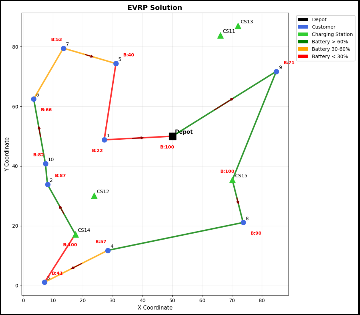
Final EVRP solution

Visualization is one of the most valuable debugging and analysis tools in routing optimization because it allows researchers and practitioners to quickly identify inefficient routing patterns, excessive charging behavior, or unexpected solution structures.

Extending the EVRP Framework

The current EVRP implementation captures the core routing and battery feasibility challenges involved in electric vehicle logistics. However, real-world transportation systems are significantly more complex and dynamic. The model can therefore be extended with several additional operational features to make it more realistic and applicable to production-scale logistics environments.

The basic EVRP model could be extended with more real-life features like:

• Multiple vehicles
• Time windows
• Fast vs slow charging
• Dynamic traffic
• Real road networks
• Stochastic energy consumption

The Electric Vehicle Routing Problem introduces a new level of complexity to classical routing optimization by incorporating energy feasibility into route planning. Unlike traditional vehicle routing models, EVRP must balance operational efficiency with the physical constraints of electric mobility.

In this article, we developed a complete EVRP optimization pipeline. The implementation goes beyond solving a single static routing instance by providing a flexible and extensible framework capable of generating synthetic datasets, constructing optimization models, solving routing problems, validating solution feasibility, and visualizing routing behavior.

The project highlights an important idea in modern optimization engineering, where solving the optimization model itself is only one part of the overall system. Practical decision-support tools also require:

• Data generation and preprocessing
• Solver management
• Feasibility verification
• Result interpretation
• Visualization and reporting

These surrounding components are often just as important as the optimization formulation itself when building deployable decision systems.

Overall, we provide a practical implementation of EVRP and a foundation for exploring larger and more advanced routing optimization problems in intelligent transportation and logistics systems.