Geometric computer vision with Mathematica

I’ve spent huge amounts of time using Mathematica, in part because I found Mathematica Stack Exchange to be such a great community, and in part because I found Wolfram Language to be incredibly interesting, fun to play around with, and just different from other languages. However, there’s one thing that Wolfram Language has always missed, which has annoyed me since I started working professionally with computer vision, nine or so years ago. That is functionality for geometric computer vision.

Mathematica 15 was released a few weeks ago and with that came an MCP server. Combine that with the quite recent maturation of generative AI models for coding, and it seemed to me a great opportunity to build my own packages for computer vision using Codex. In this article, I’ll write about my attempt to do so, and in the process, we can all get a feeling for

1. How well Codex (ChatGPT 5.5 and ChatGPT Terra with the effort level extra high) works with Wolfram Language and the new MCP server.
2. What packages for geometric computer vision could look like in Wolfram Language.
3. What the packages might be used for, since I’ll create a few demos that I’ll share in this article.

If you have no idea what I might be referring to when I say “geometric computer vision”, here’s an overview:

• Camera calibration: Finding the camera parameters required for a camera model.
• Camera models: A mathematical device to simulate image formation. For example, if a photo is taken of a scene with 3D points in it, where do the 3D points end up in the image? Or if a landmark is seen in the image, along what ray would it appear in the 3D world?
• Camera pose estimation: Given 2D points in an image, belonging to a known object, what is the camera pose relative that object?
• Epipolar geometry: If there are two cameras, epipolar geometry tells us e.g. how points and lines in the view of the first camera will show up in the view of the second camera. Also, given points and lines in 2D, what can be said about the relative pose between the two cameras?
• Triangulation: Given corresponding 2D points in different camera views, what are the corresponding 3D points?
• Bundle adjustment: Given corresponding 2D points in different camera views, simultaneously estimate camera poses, camera parameters, 3D points, and possibly even refine the 2D points.

This functionality already exists in libraries like OpenCV, but, as mentioned, not yet in Wolfram Language.

To demonstrate the packages that I’ve created, I’ll go through some of the use cases mentioned above, and show how to solve these problems with the packages.

Prerequisites

The packages that I will be demonstrating in this article can be downloaded using the link below:

• Geometric computer vision Wolfram Language packages

The code is split into multiple packages to make it easier to handle. In the rest of the article, I shall assume that the symbols from all the packages have been imported into the global namespace.

If a notebook is placed at the root of the unzipped archive linked to above, the loading of the symbols can be done like this:

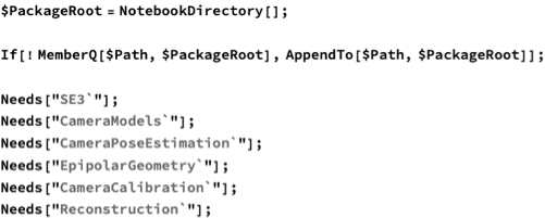
Whenever I reference a package in this article, it’s one of these packages.

Camera calibration

Camera calibration is perhaps the most fundamental functionality that a geometric computer vision package must have. The package must provide two things:

• Camera models that map 3D points to image pixels.
• A way of fitting the parameters of the models. The parameters are often thought of as two different groups: Six parameters that encode the pose (translation and rotation) of the camera in the world coordinate system, and any number of parameters that encode the transformation of 3D points in the camera coordinate system to 2D pixels.

The package supports the same camera models that OpenCV supports. One is a pinhole camera model with a flexible distortion model, which at its simplest is a Brown-Conrady distortion model, but which, when more parameters are used, turns into the so-called rational distortion model. The second camera model is the Kannala-Brandt camera and distortion model, which is designed for fisheye cameras.

To calibrate the models, we need images of a known calibration pattern, seen from different angles. Here are some of the ones that I recorded with my webcam for the purpose of this demo:

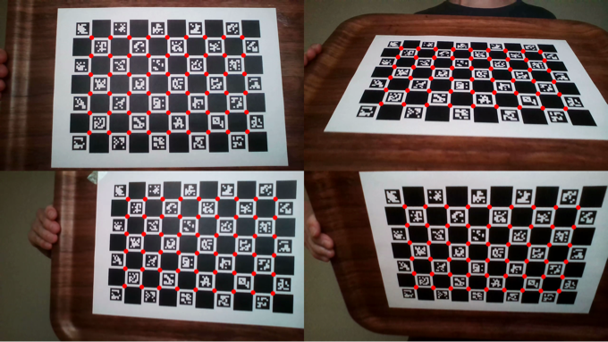
Images taken with a webcam of a Charuco pattern taped to a flat surface. Red dots show corners detected with OpenCV.

Checkerboard patterns are typically used because the corners are easy to detect. Aruco patterns are often combined with checkerboard patterns because 1) it makes the orientation of the pattern distinguishable, and 2) the pattern can be used even if it’s only partially visible.

I wrote Wolfram Language code for detecting Aruco patterns in an earlier post: Aruco Marker Detection.

OpenCV provides the means to generate the patterns and to detect the corners in the images, I did not use my own implementation for that. However, with the package that I created, we can calibrate the camera model purely in Wolfram Language, like this:

Where targetPoints is a list of 3D points representing the corners in the target coordinate system, and imagePointSets is a list of 2D corner positions for all the 21 images used for the calibration. And we can inspect the result:

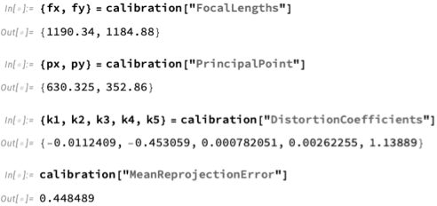
Just like that, we have all the camera parameters that we need for the pinhole camera model with the Brown Conrady distortion model. The reprojection error is less than half a pixel, which indicates that it found a good solution. Also, the difference between this solution and that of OpenCV is less than 10^-5 for all parameters. The difference in the mean reprojection error is only 10^-8. This shows that the Wolfram Language implementation, using FindMinimum underneath, finds the same solution.

Projection and backprojection

The most fundamental operation of a camera model is to project a 3D point onto the camera image, and to take a point in the camera image and backproject it. When backprojecting, we don’t get a 3D point since we don’t know from a single image what the depth of the point is, but we get a ray in 3D, and we know that the point is somewhere along that ray.

With the package, projection is done like this:

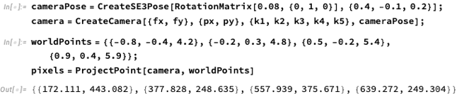
We can turn the pixels into rays in the camera coordinate system using BackprojectPixel, like this:

And we can get the rays in the world coordinate system like this:

Those that have studied geometric computer vision also know that the plane where z = 1, called the normalized plane, is of special importance. The points can be retrieved in this plane using UndistortPixel:

Whenever we go from a pixel to 3D, we always need to undo the distortion, that’s why the function is called UndistortPixel.

The distortion can also be removed from the image itself using the function UndistortImage:

The webcam didn’t have a lot of distortion so the difference isn’t very big, but it would still be significant in computer vision projects that require high accuracy.

Qualitatively, the difference looks like expected. The distortion is radial and increases with distance, so it’s going to be the smallest in the center of the images. Additionally, shifting pixels in uniform parts of the image isn’t going to make a significant difference.

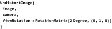
There is another function that UndistortImage can perform, which is conceptually interesting. We can not only remove the distortion, but also rotate the camera and resample the image with the new camera angle. This results in an image that looks as if it were taken from that camera angle.

It works like this:

• For each pixel in the new image, backproject the pixel to a ray.
• Rotate the ray the same way that the camera has been rotated.
• Project the rotate ray onto the original image and get the color.

A real-world application is the birds-eye view parking display found in modern cars, which takes camera images that are pointed towards the ground, at an angle, and resamples the images as if the cameras were looking on the ground from above.

This is what a typical call utilizing this feature looks like:

SE(3) poses

A pose consists of a translation and a rotation, and they are of fundamental importance in geometric computer vision. Each camera has a pose within the world coordinate system, and any objects in the camera images have poses that we can infer relative the camera pose, also known as the camera coordinate system. For this reason, the package provides functionality for composing poses, inverting poses, and transforming points between coordinate systems given by poses.

This is what it looks like:

Note how the dot product provides a shorthand for PoseCompose. PoseMatrix returns the homogeneous matrix representing the pose.

One common operation is to transform a point from one coordinate system to another. It can be done like this:

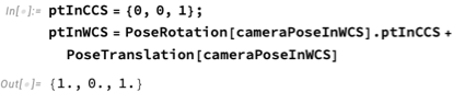
Or using the homogeneous matrix:

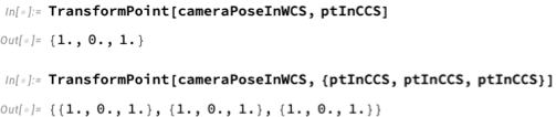
But since this is a common operation, there’s also a helper function for it:

Pose estimation

A common task in geometric computer vision is to determine the pose of an object relative the camera, or, equivalently, the pose of the camera relative the object. The former is usually known as pose estimation, whereas the latter is known as extrinsic camera calibration, because we are in this case determining the pose parameters of the camera model.

While the pose of any type of object can be estimated as long as there are 2D landmarks that can be detected on it and the corresponding 3D points in the object coordinate system are known, a simple example is the Charuco calibration target used for intrinsic camera calibration earlier:

The drawn coordinate system shows the pose estimated by the camera pose estimation package.

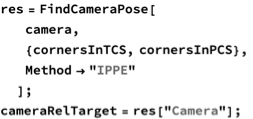
To get the pose, we start by using OpenCV to get the 2D pixel coordinates and the corresponding 3D points in the target coordinate system (which is the one visualized above). We shall call these cornersInPCS (PCS = pixel coordinate system) and cornersInTCS (TCS = target coordinate system), respectively.

We then estimate the pose like this, using IPPE, which is an algorithm designed for planar objects:

Then, the visualization is done like this (this demonstrates ProjectPoint with an actual use case):

This piece of code results in the image already posted.

For objects that are not planar, FindCameraPose also supports P3P with RANSAC and EPNP. After having found the initial pose with either of these methods (P3P, EPNP, IPPE), it refines the pose by minimizing the reprojection error with a nonlinear least-squares optimization (FindMinimum).

One application of pose estimation is augmented reality, as seen in this following video:

[embed]

This video has been a long time coming. After writing my article on how to detect Pokémon cards, eight years ago, I wanted to put 3D models of Pokémons on top of the cards as well. However, Mathematica didn’t support importing 3D models with colors and textures, and so I wrote my own package for that. Unfortunately, I never wrote the article that was supposed to use it.

Epipolar geometry

Given two images of the same scene but from different angles, it’s possible to say something about where a point in one image will show up in the other, without fully estimating the relative pose between the cameras that took the images. This type of geometrical insight is what’s known as epipolar geometry, and it typically proceeds like this:

• Find corresponding points between the two images. This can be done using image descriptors such as SURF, ORB etc. The methods for finding corresponding points come built into Wolfram Language in the form of ImageCorrespondingPoints.
• Estimate the fundamental matrix F or the essential matrix E.
• Use either of the constraints x E x’ = 0 or x F x’ = 0, where x and x’ are corresponding pixel coordinates in the two different images.
• If x is given, the constraints trace a line in the other image. This is the most we can tell without knowing the camera poses exactly: that the point x in the first image will appear along the line E x’ (or F x’) in the second image.

Finding corresponding points is, as mentioned, easy with the built-in ImageCorrespondingPoints:

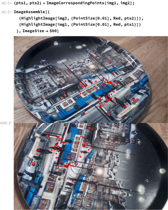
The package provides FindEssentialMatrix and FindFundamentalMatrix, which use the eight-point algorithm with RANSAC to estimate the matrices.

If we follow the procedure outlined above, we should be able to pick a point in the first image, and find a line — the so-called epipolar line — along which it should appear in the right image.

Here is the code for doing this:

The yellow markers are corresponding points. Given the position of the yellow marker in the first image, a contour plot of the constraint traces out the red line in the second image, which as can be seen passes through the yellow marker.

It is also possible to partially recover the relative pose from the essential matrix, and the package provides the function RecoverCameraPose for this purpose:

However, the translation of the pose has unknown scale. Only the direction from one camera center to the other camera center is known, not the distance.

Reconstruction

Reconstruction in geometric computer vision is the process of creating, from a set of images, a 3D representation, such as a point cloud, Gaussian splatting, or a mesh.

The reconstruction package has utilities to support creating a point cloud from images, that which conceptually is known as structure from motion (SfM). Structure from motion proceeds like this:

1. Detect corresponding 2D coordinates between images.
2. Estimate the camera pose relative each image (we have already seen how to do this for a calibration target in an earlier example).
3. Using the estimated camera poses and the corresponding 2D coordinates to triangulate 3D points.
4. Running bundle adjustment to jointly optimize the 3D points and the camera poses.

The reconstruction package helps by providing a function called FindImageCorrespondences that can be used to implement (1). It is like the built-in ImageCorrespondingPoints, but unlike that function, it can detect correspondences across an arbitrary number of images, not just two.

It also provides a function called TriangulatePoint which can be used to triangulate points given a list of cameras and a list of 2D coordinates. This can be used to implement (3).

Finally, it provides a function called BundleAdjust that can be used to implement (4).

To demonstrate this, I will create a 3D model of my own face, which I will then use to implement head tracking.

For the first step, getting 2D detections, we will use Mediapipe in Python. In principle, we could have used the 2D face alignment net from the Wolfram Neural Net Repository, but it’s not accurate enough, so I’m going with the Mediapipe solution instead.

I have a collection of frames from a video taken with the previously calibrated webcam, with different head poses. When I get the 2D face landmarks with Mediapipe, this is what it finds:

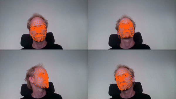
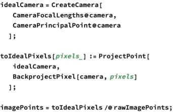
Assuming that rawImagePoints are the 2D detections seen in those images, the following code defines a new variable, imagePoints, that’s the same set of points without lens distortion.

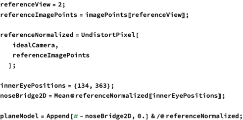
We are now at step (2), getting an initial pose for each image. It might seem like we can’t use FindCameraPose because that requires 3D-2D pairs, and we don’t have 3D points yet. However, we can use a planar approximation to get approximate poses:

1. Pick one image and call this the reference image.
2. Assume that all face points are on a plane in 3D. If this assumption were true, then the detections in any image will be related to the detections in the reference image by a homography.
3. Find the homography to the reference image and extract the relative pose from it. This is what IPPE does, but in a way that’s more robust than directly constructing the relative pose from the homography matrix.

Of course, the assumption that the points are in a plane is wrong, but it will give us a starting point. We will refine the poses later.

When later using the 3D head model for head tracking, we’ll want the head model to be defined in a sensible way. I’ll use the landmarks of the inner corners of the eyes to find the nose bridge, and use that as the origin of the coordinate system.

The code looks like this:

The next step is to find all the poses relative the reference:

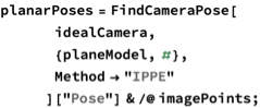
And once this is done, we can now find the poses for all the other images relative the reference. Once we have all the poses, we can triangulate the 3D points in the head model:

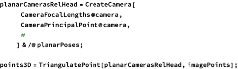
Which can be visualized like this:

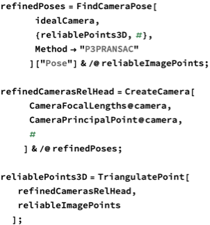
We now have 2D-3D pairs and a set of poses, so we could move on to bundle adjustment. However, some face landmarks may be more unreliable than others. We can make the head model more reliable for the purposes of head tracking by removing those points from the model:

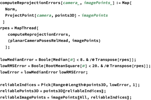
After this, we can refine the poses and the head model using only the reliable points:

Finally, now that we have a guess for 2D-3D pairs and poses, it’s time to run bundle adjustment to jointly optimize the 3D points and the poses:

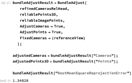
This results in a low reprojection error, especially considering that the 2D landmarks are bound to have noise.

Let’s visualize the final points. This time, color is used to emphasize the depth difference across the points:

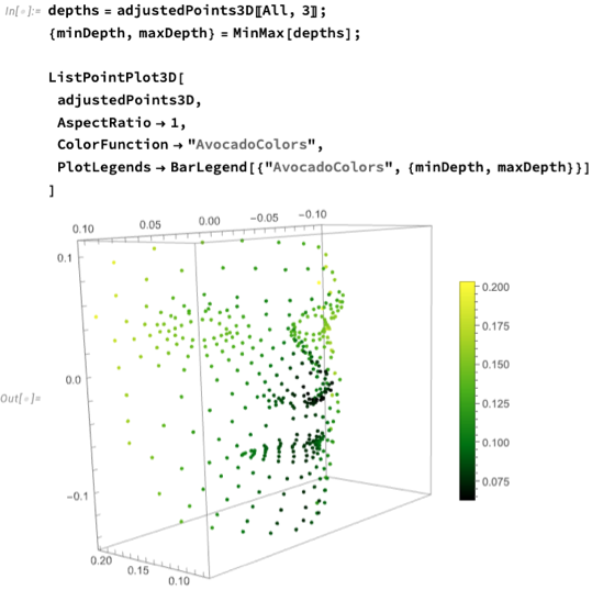
We can now implement a function that takes 2D detections from an image and returns the head pose:

P3PRANSAC is used rather than EPnP, which FindCameraPose also supports, because RANSAC makes it more robust to bad 2D detections.

It should be noted that although the rotation of the head will be correct, the translation will not be entirely correct because the head model is only known up to scale. This is an inherent limitation with a monocular camera system. A larger head further away from the camera looks the same as a smaller head closer to the camera, so it’s impossible to say how far away or how large the head is. With a multicamera system, this could be resolved.

Conclusion

The goals for this article, as stated in the introduction, were threefold:

• Test how well Codex works with Wolfram Language.
• Explore what packages for geometric computer vision might look.
• Demonstrate use cases for the packages.

The article largely speaks for itself when it comes to the two latter bullet points. As for looking at this as an exploration of how a package for geometric computer vision might look, it should be said that the naming of the functionality is not always according to the normal conventions for built-in functions, and e.g. the choice of having functions that create expressions is not how it would have been implemented if it were a built-in set of functions. The point of functions such as CreateCamera that create an expression with the head Camera, is that Camera doesn’t do validation of the input, but CreateCamera does.

However, if we zoom out from the details, and look at the big picture, we can see that the packages provide a set of functions that work well together, and also with built-in functions, to accomplish practically useful tasks in geometric computer vision.

Regarding how well Codex works with Wolfram Language, I made these observations:

• I could always stay within Codex. I never needed to look at the code. That’s not to say that I didn’t need to know how things were implemented, but I could ask about that rather than looking at the code.
• When looking at the code, I noticed that it’s often not written the way I would have written it. Wolfram Language requires a lot of deliberate effort to make code readable, and Codex — or rather, the models used — could do better in this regard.
• When asking it about options for how to implement something, it always knew everything. However, when asking it to implement something without specifying how, it often started by implementing something that was either algorithmically inefficient or inefficient because of how it was implemented, e.g. not vectorized. That is why it was important to ask about the implementation, to guide it directly by saying how something should be implemented, or to ask it for options on how to improve the code, and then ask it to implement the suggestions that are desirable (not all are — some might increase the complexity a lot for a small gain, for example).
• It seems to prefer simple solutions first, but is capable of implementing more complicated solutions if asked for it. For example, when implementing BundleAdjust, it first used FindMinimum to solve the optimization problem. However, when pushed to make it more efficient by utilizing the sparse structure of the normal equations, which is inherent to bundle adjustment problems, it implemented its own sparse solver (utilizing LinearSolve as appropriate).
• Developing demos was very useful for improving the code. If something took longer than expected, one could ask Codex to benchmark the code and then have it iterate to bring the speed down. It sometimes presented options with different levels of complexity, so that I could have a say in the trade-off.
• The fact that one has to involve oneself, and manually push for optimizations, means that different parts of the packages are optimized to different degrees. The level of optimization depends to some degree on how computationally heavy the use cases for those functions are, in general, but also on the problems that I selected to evaluate each of them on.

What this experience shows is that one can’t just ask for something and expect to get production ready code. While Codex does not always produce production ready code, Codex can, however, be a help in creating production ready code. It has the knowledge about possible implementations and so on, it’s just not certain that it chooses to implement the best solution for production.

For ad hoc work, where perhaps one wants to experiment in a new area, but don’t care about production quality, Codex is great. Codex will create something that works, and if one later runs into a use case with efficiency problems or something else, then Codex can improve the code to handle that particular use case better. That’s all one needs for ad hoc work — a solution that works for the problem at hand, and Codex is great for that.

Importantly, the issues with Codex generated code is almost always efficiency or robustness (e.g. one might have to prompt it explicitly to handle noise in the input), not correctness. The area where it struggles the most with correctness is with visualizations, where it’s sometimes unclear if it understands what the problem is visually or not — although it will say that it does — , and in trying to solve one visual problem, it might introduce another without noticing.

I think that the most important conclusion from this experiment is that whereas before, using Wolfram Language for certain domains seemed impossible, because first writing a package for all the basic functionality needed, and then working on the problem one actually wants to work on, would take too much time. Now, with AI able to help out a lot, especially for ad hoc work, using Wolfram Language in domains that are not support by built-in functionality or publicly available packages has become much more feasible.