A Simple Non-Malthusian Model

[This is part of my series on Thomas Malthus’ “Essay on the Principle of Population,” first published in 1798. You can find an overview of all my posts here that I will keep updated: “Synopsis: What’s Wrong with the Malthusian Argument?” — Note that this is a work in progress, my previous posts may be outdated and contain errors. Later posts supersede earlier ones.]

I would like to present a very simple model for population dynamics here that is non-Malthusian in the sense of my previous post. By “non-Malthusian” I mean roughly that a population with such population dynamics will not regularly end up in a Malthusian endgame with maximum population size (or equivalently: population density for fixed area) and with a minimum for the food supply per capita.

If the Malthusian endgame does not regularly materialize, the implication is that populations stabilize their sizes well below a maximum where mortality begins to rise steeply because the food supply becomes insufficient and people simply starve to death. Stabilization could also result from other factors than the food supply which lead to rising mortality with more population. For example, more frequent outbreaks of epidemics or higher levels of aggression, as with wars and civil strife, could force stabilization via rising mortality already before a population enters the Malthusian endgame.

However, such a theory no longer necessarily is a Malthusian theory of population dynamics in my sense. The food supply might never play a role as a binding constraint if other factors regularly stop population growth already before the Malthusian endgame is reached. The theory is only Malthusian if the level at which a population would stabilize because of such factors lies regularly above that in the Malthusian endgame. Effectively this means that either it is an exception or otherwise we have a non-Malthusian theory of population dynamics.

But then I make a much stronger and truly non-Malthusian assumption here, namely that rising mortality does not determine the level where a population stabilizes. Even stronger: My premise is that mortality does not vary in population size at all, though it may change for other reasons. That is not implausible as historical data support a view that mortality is more or less fixed under pre-modern conditions, effectively like a constant of human nature. There was, of course, considerable variation over the short term, but it was not obviously related to population size as should be the case in a Malthusian theory of population dynamics, at least at the upper end of the range where the population approaches maximum size and runs into a hard constraint from the food supply.

Now, if mortality is independent from population size, it cannot stabilize a population. That can only happen via changes in fertility. For this to be the case, fertility has to go down low enough that it reaches the replacement level for given mortality where as many new children are born as people die. Fertility does not have to remain exactly at the replacement level for stabilization. It is entirely sufficient that it behaves in such way that it counteracts deviations from the stable level. Fertility might hover or, even more regularly: oscillate around it.

All it takes in this case is that fertility goes below the replacement level when the population is above the stable level and above the replacement level when it its below it. This turns the stable level into a fixed point for the dynamical system. Since there is population momentum, we also have lags of about two generations for the effect of fertility decisions in the past on current developments. This can lead to phenomena like overshooting above or undershooting beneath the stable level that need to be corrected to achieve stabilization. Together with other deviations from the target, eg. random fluctuations, movements for population size around the stable level have to die down and not blow up over time to make it work.

— — —

Malthusians would challenge the very idea that stabilization via fertility was possible in pre-modern times. In their view, populations always had fertility well above the replacement level, something that is suggestively called “natural fertility,” in Malthus’ original argument: even close to a maximum that is biologically possible. If that were so, the Malthusian endgame would be inescapable except temporarily in special cases like initial settlement, technological progress for food production or severe setbacks for a population caused by catastrophes.

To strengthen the point, Malthusians would also point out that there is little evidence for wide-spread birth control in pre-modern times. However, that is somewhat of a red herring. They themselves have to resort to other explanations for variable fertility when they have to reconcile actual data with a claim of very high, even maximum fertility in the past. Already Malthus thought that varying age at marriage could modify fertility somewhat, also that the expectation of hard times for someone and their children could lead to lower fertility or even only the expectation of a lower status in society for one’s descendants. He also insinuates at some points that the supposedly fixed level for fertility close to a maximum might not be as fixed in some cases, eg. when he discusses Native Americans who he suggest are rather apathetic about sex.

Nonetheless, he passes over the possibility that these behavioral changes together with others he has not in view could also go so far that they can also bring the replacement level within reach for a population. If that were feasible, population growth could stop because of fertility alone and the Malthusian endgame would be called of.

As I will show below, it is by no means clear that pre-modern populations could not modify the level of fertility enough to make also population stabilization possible. Actually, such populations were able regulate their fertility well enough, however that worked, that the regular level remained far below a maximum, and much farther away from it than from the replacement level. Now, if the large step down from the maximum is possible, it is not obvious why the small step further down to the replacement level should not have been possible, too.

And indeed, historical data make such a conclusion unavoidable as populations often stabilized at levels without a Malthusian endgame playing out or even shrunk at times with no dramatic increases in mortality that could be the explanation. I would even strengthen this claim: It is dubious that a Malthusian endgame ever materialized except in situations where the food supply collapsed suddenly and unexpectedly.

In this post, I do not pursue the question further how fertility could be regulated to such an extent with no obvious wide-spread birth control. Instead I just assume here that sufficient control over fertility was possible, which need not mean that this was a conscious activity alone. My suspicion actually is that this is a mechanism at base that is more or less hard-wired.

If stabilization occurs because of fertility, the conclusion has to be that it must go down with population size, at least in a relevant range. Or in other words: Fertility must be density-dependent because as noted above, for fixed area, population density is equivalent to population size. That is the basic idea behind the model I am about to develop.

— — —

My first idea was that fertility might be a decreasing linear function in population size. The population will then stabilize at the level where the linear function hits the replacement level. The reason for this functional form was that the mechanism might plausibly be hard-wired into human nature. And if so, it should require only simple computations in the background. Moreover, my intuition is that also many other species pursue similar population dynamics as I assume humans do. That could not be so if the underlying mechanism depended on higher functions unique to humans.

However, when I looked at data for actual populations I became convinced that the functional form is different. This conclusion dropped out of an analysis for population dynamics in South Korea over the 20th and early 21th century. In this case it looks as if there is a linear relationship not between fertility and population size, but between the logarithm of fertility and the logarithm of population size. That has a certain logic to it because the logarithm makes complementary percentage changes symmetric: An increase by 100% is the same as minus a decrease by 50% (not 100%), so they cancel out as would do the percentage changes. Logarithms are harder to calculate, but then this is not an insurmountable obstacle for a hard-wired mechanism as logarithms are also used in the auditory system.

If you transform a linear function for the logarithms back with the exponential function, you obtain a power function for the relationship between fertility and population size:

A power function should be even easier to calculate than logarithms, a linear function and an exponential function. You could, for example, exploit its scaling property to do that. To this end, you could start with a small step, eg. by 1%. The scaling property amounts to this:

Factors that are plugged into the function, come out as a power. All you then have to know is some starting value and the fixed factor before p(x). With that, you can calculate a sequence of values on a logarithmic scale, which should do the trick. Note that I do not assume that anybody does that on a conscious level. What I am thinking of is some hard-wired mechanism that does the calculation for you in the background. My speculative idea is that this calculation piggybacks on some other essential mechanism that yields the result. If that were so, this would immediately yield an argument why the functional form is stable under evolution because changing it would require changing an essential mechanism that just cannot be changed without serious side effects.

The exponent of the power function is the slope of the linear function for the logarithms of the two variables. I estimated that this slope for South Korea, respectively the exponent, is about -1/0.3 = -3.33 (cf. my article here). The relationship then appeared to be of the following form, with TFR for the total fertility rate and DENSITY for population density (or for fixed area population size):

The constant R is a reference level for population density or size, in my initial derivation: the stable level. The constant C is the inverse of the replacement level for fertility that appeared on the lefthand side.

Note that both quantities need not be constants, but might also be variables that depend on other factors. Obviously, the replacement level is determined by mortality. And as for the reference level for population density, my intuition is that it should reflect a measurement for how well the population is doing. I call this the “level of distress.” As distress goes up, R goes down, as it goes down, R goes up. My tentative conclusion is that this “level of distress” turns around the longer-term nutritional situation and various proxies for it. It also seems to be an estimate for a volatility, though I have to stress that all this is not the final word yet and speculative.

Since I assume that the above relationship does not depend on the specific population, but is a part of human nature, I take it as the basis for my model below. Data for Japan support a conclusion that this behavior might be a general feature for humans. I picked those two countries for my derivation because they have had very little immigration and emigration that might affect population dynamics. Countries with immigration have had population growth much greater than for countries without it. If the general logic is sound, the stable level must move upwards with immigration even without a change for the “level of distress.” Or else, for example, the population of the US would always try to return to some lower level, which cannot be true.

— — —

One mistake I perhaps made in my original derivation was to assume that stabilization would have to be at a level independent from mortality. That created a puzzling problem. To stabilize population sizes always at the same level, a population would have to aim for the replacement level that depends on variable mortality and is hence also variable. It must be higher for high mortality because, as more people die, more have to be born to keep the population stable. But it was unclear how a population could track changes for the replacement level because that is not directly observable.

However, it is not necessary to assume that mortality does not play a role in determining the level at which a population stabilizes. All I need in the current context is that it is independent from population size while it could well depend on other factors or just change randomly. In retrospect, I may just have gotten this point wrong. As soon as you drop the requirement that the stable level has to be the same for any mortality, things become considerably easier. All it takes is that the population stabilizes, not that it stabilizes always at the same level. That is the idea behind my model now.

As pointed out above, I assume that there is a fixed relationship between fertility and population density, or equivalently for fixed area: population size, that has the following form:

In addition, I assume that the two values C and R are constant and not variable. That makes one of them redundant because it can be packed into the other one. We can hence simplify the relationship with a constant R’ to:

This is a power function with a pole at zero, ie. its value goes to infinity there. It falls off to zero as population size increases to infinity. Here is a plot for the function somewhat away from the pole:

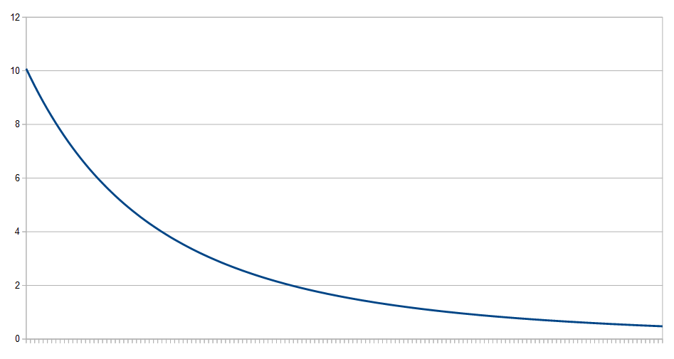
The eventual decay to zero effortlessly yields that the function must fall to the replacement level for any given mortality. This is so because the replacement level can never go below two. As long as people die, they must have at least two children per woman to keep a population size stable, so two is a lower bound that can never be breached.

However, the value at which the function hits the replacement level now depends on mortality. If mortality is higher, so is the replacement level. You can then find the corresponding stable level by taking the replacement fertility on the Y-axis, going to the right until you hit the curve, and reading off the level on the X-axis. Obviously the relationship is that higher mortality implies a higher replacement level and then a lower stable population size and lower mortality implies a lower replacement level and a higher stable population size.

That is already essentially the whole model here. In my program in the background, I make a slight adjustment. Since I work with population size directly and want to avoid divisions by zero, I add one to population size, which moves things slightly away from the pole. The resulting deviation is minimal as I work with population sizes far above a few people.

The rest is only to make assumptions about mortality, which then implies a level for the replacement level and the level at which the population stabilizes, as well as for fertility, ie. when people have children and with what probabilities. Once you have that, you can simulate the behavior of a population with such population dynamics.

— — —

Let me now spell my assumptions out for the inputs to my program. I do not aim for photorealism, but only for moderately realistic parameters that stay close to values for actual populations.

As for mortality, I take data for Germany, and for a reason I will explain below, two sets of them. The first input is mortality for Germany in the decade from 1870 to 1880, ie. when Germany was still a mostly pre-modern country. Compared to other countries at the time, mortality was pretty high. Here is the function for survivorship:

You have to read the graph in this way: On the horizontal axis is age for a person. On the vertical axis, the curve starts out at 1, ie. 100%. It then falls off in this way: Of the 100% initially, what share is still alive at the respective age?

Most of the mortality comes in the first five years, especially in the first year. This was brutal. Of the 100% at birth, 25% died until age 1. Then mortality slowed somewhat down. Nonetheless, after five years 35% of the initial 100% were dead. Until age 15, 39% had already died. If someone had made it through this horrible early phase, mortality became comparably moderate. Only at higher ages did it speed up again, and at age 100, practically everyone was dead.

Mortality at such a level corresponds to life expectancy of only 35.1 years. However, as you can see, the naive interpretation is wrong that this meant hardly anyone lived past age 40 years. True, many died in the first few years, but those who survived had a good chance to live to ages far beyond 40 years. Even ages of 70 or even 80 years were in reach for many of them.

— — —

As my second input, I take modern data for Germany, now in the years from 2016 to 2018. Here the graph for survivorship looks quite different:

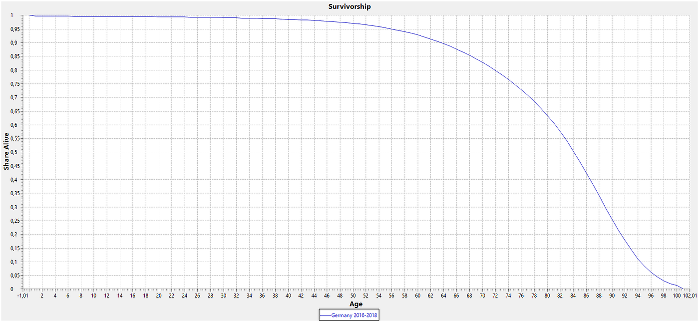
It is still so that the first year is particularly risky, but by no means on the level as in the 19th century. Once you have made it past that, your chance to die is very low until perhaps age 50. Only then does mortality speed up, but also more slowly than in the past. Life expectancy with this level of mortality is considerably higher, namely 80.4 years. (Note that I have averaged it out for men and women in both cases. I also leave ages above 100 years out, which are still rare, but would pull the average slightly up.) While people also die less frequently at higher ages, the big change has been the spectacular decrease for child and especially infant mortality. All in all, a much higher share live to ages 70, 80 or even 100.

— — —

I now turn to fertility where I don’t use actual data, but a rather stylized functional form. Here is the graph for hazard rates, the chance of having a child:

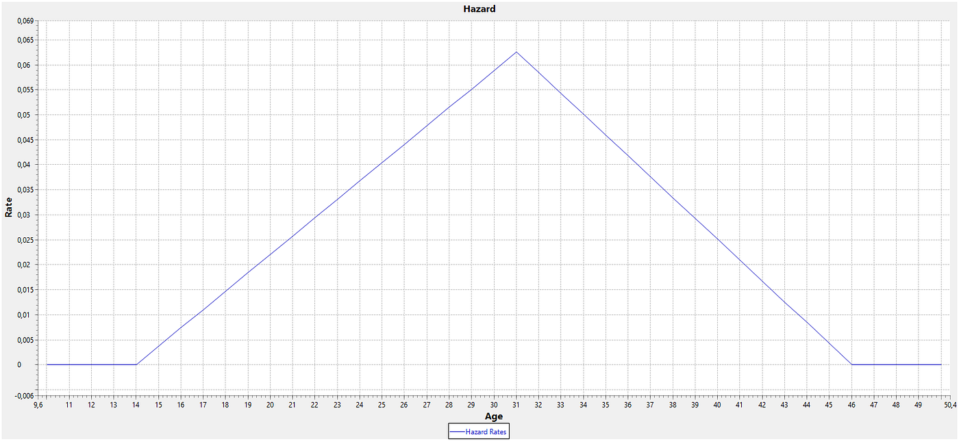
The graph shows the probability that a woman at a certain age, on the horizontal axis, will have a child in a given year. The function increases linearly from zero at age 14 to a maximum at age 31. It then falls off also linearly from there to zero at age 46. As noted, this is not exact for actual populations, but still roughly realistic for Germany now. In earlier times, you also had such a triangular form, but with a peak that came in the early 20s. The shape has changed over time, especially over the past few decades, with age at birth moving upwards. I do not model this here, but assume that this functional form is fixed, which is not entirely correct for the more distant past. Implicitly my assumption leads to a generation length of about 30 years, while an earlier peak would shorten this roughly to where the peak is.

The function for hazard rates is normalized. That means if you add all probabilities up, you get 1. In other words: If women had children with these probabilities, they would end up with one child over their life, that is if they live through fertile age. However, what I want in my model is that the level for fertility can change. I achieve this by lowering and raising all those probabilities by the same factor, which is the total fertility rate that measures how many children a woman will have if she lives through fertile age. In principle, probabilities can go beyond 1 for very high factors. But probabilities beyond 1, ie. 100%, are meaningless, so I effectively cut the function off at 1 in such a case, which means that total fertility rates are lower than the factor. But for normal levels, they are the same.

With mortality, the number of children will be lower because not all women live through fertile age as is assumed in the definition of a total fertility rate. For modern mortality, the deviation is only slight as few women die until age 50. But in earlier times, the difference was stark. With mortality as in the 19th century, almost 40% of all women born would not even reach fertile age and would hence have no children at all. Also mortality during fertile age was considerable. So of all women born only about 40% would live to age 50. That’s why on average only about 40% of all women born would have the full number of children as per the total fertility rates. Others would have less, even down to zero children. So to have two surviving children that replace their parents in the next generation, the replacement level had to be much higher than two children per woman.

With mortality as for Germany in the decade from 1870 to 1880, the replacement level indeed works out to 3.7. A woman had to have almost twice as many children if she lived through fertile age so that the whole population including also those who did not live that long would effectively have two surviving children per woman who could replace the parent generation. For modern mortality, the replacement level is much lower, only 2.02. You need slightly more than two children per couple to make up for the slight losses during fertile age. (Note that these figures are not perfect because I have averaged mortality for men and women out while only that for women would be relevant for whom mortality is somewhat lower.)

I can now explain why I took two sets of mortality data. What I want to do is play a scenario through where mortality falls from pre-modern levels to modern levels over a century, which is roughly how it worked out in reality. To obtain intermediate mortalities, I just interpolate linearly between the two survivorship functions where a parameter of zero corresponds to pre-modern, a parameter of one to modern mortality. That is not perfectly exact, but still captures the general development. Here is how this interpolation translates to life expectancies:

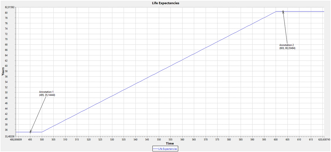
The relationship between the interpolation parameter for mortality and life expectancy is almost linear and so the increase for the latter is approximately a linear function in a scenario where the transition plays out over a century from year 500 to year 600.

— — —

If you think about it, the general development in this case is clear: Falling mortality results in falling replacement levels for fertility. If you plug that into the graph above, you then obtain rising levels for population size. The interesting part is not this result, which is in a way obvious, but how the population dynamics of the model play out.

To study this, I can now run a simulation with these inputs over centuries. Since I start with an population who are all born in year 0, the population starts out in a weird way with fertility shooting up to an absurd maximum level, basically turning all probabilities up to 100%. It then takes a little to stabilize. Since that is more of an artifact, I don’t show this early part in the following graphs, but start out somewhat before the transition for mortality gets going in year 500. Here are population sizes over time where I average out over 1,000 simulations, ie. this is like a population in the hundred thousands:

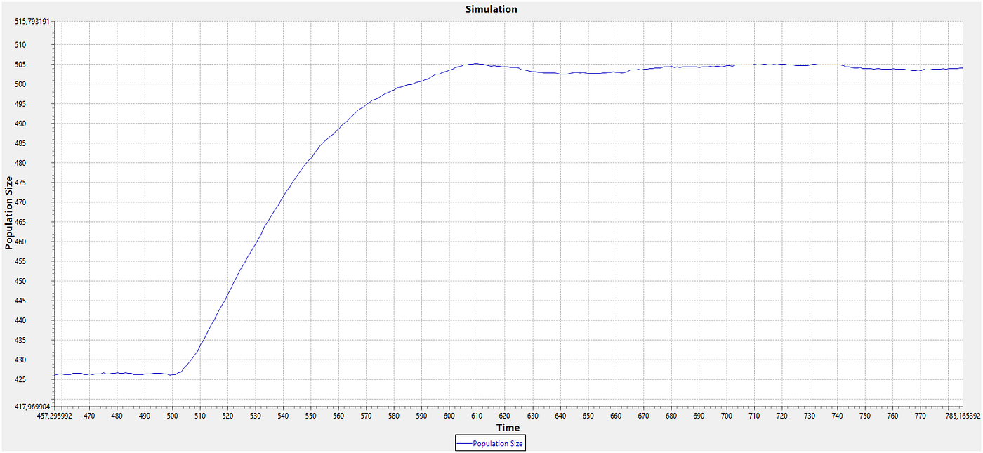
The population has stabilized at a level slightly above 426 before year 500 (I have set the constant R’ to 500). As mortality falls, the population size increases almost linearly. But then growth slows down after about half a century. Population sizes reach a peak of 505 slightly after the transition in about year 610. From there they fall slightly, but recover again. There are slow oscillations with a length of four generations or about 120 years that die down at a level somewhere between 503 and 504. All in all, population size increases with the transition from pre-modern to modern mortality by about 18%.

The oscillations after the transition are slight and only visible if I zoom in on the period from about year 600 on:

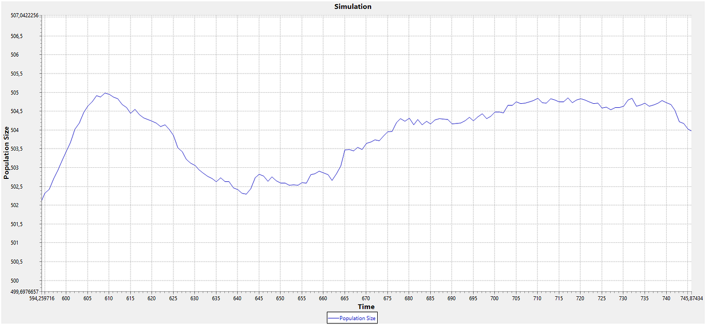
There is some overshooting when the mortality transition comes to an end, which then gets corrected down, but somewhat too much. That then leads to a further correction upwards, then downwards, and so forth.

Let’s now look at how the transition works out more in detail. Here are annual growth rates, which are somewhat wiggly because this is a simulation that involves some randomness:

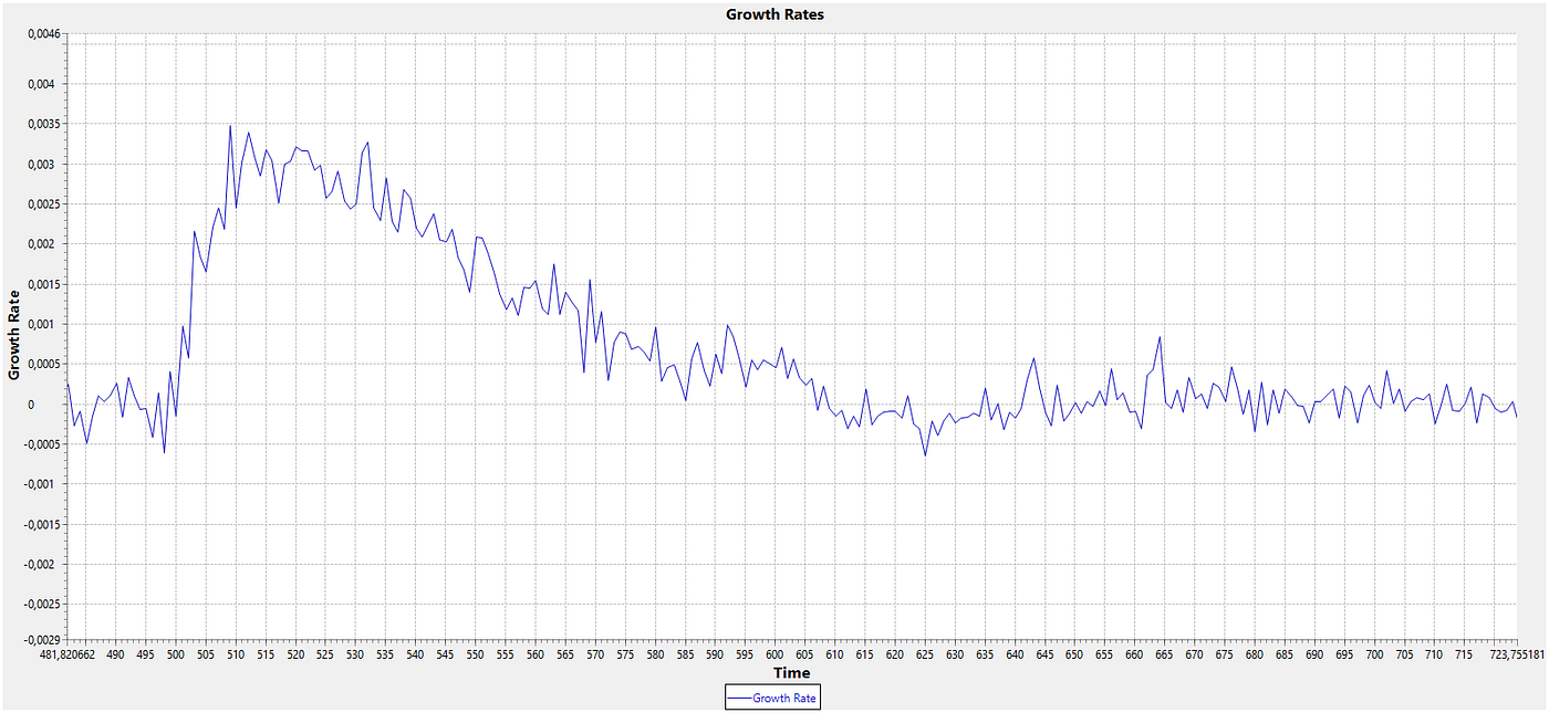
The graph shows a behavior that corresponds to the development for population sizes. Before year 500, growth rates jump around a level of zero because this is a stable level for high pre-modern mortality. However, as mortality starts to fall, growth rates initially ramp up to about 0.3% per year, then fall slowly back to zero. If you look closely, you might also see the oscillations. But they are hard to track in all the noise.

Here is now a view on total fertility rates for the population that is easier to read:

The blue curve is for actual total fertility rates in the simulation, the red curve for the respective replacement levels. The latter fall roughly, though not exactly linearly from the higher level for pre-modern mortality of 3.7 to the lower level for modern mortality slightly above 2.

As you can see, actual total fertility rates go somewhat above the replacement level at the start, but then fall below it. Only later do they converge to the low level for modern mortality. You can view this is a slow oscillation overlaid on the transition for replacement levels. Fertility below the replacement level along with population growth is perhaps somewhat counter-intuitive. However, the explanation is simply that a population can also grow because people live longer with falling mortality. And this effect is apparently stronger than the effect from below replacement fertility.

We have again similar oscillations for total fertility rates as we had for population sizes. I again zoom in on the later phase after the transition from about year 600 on:

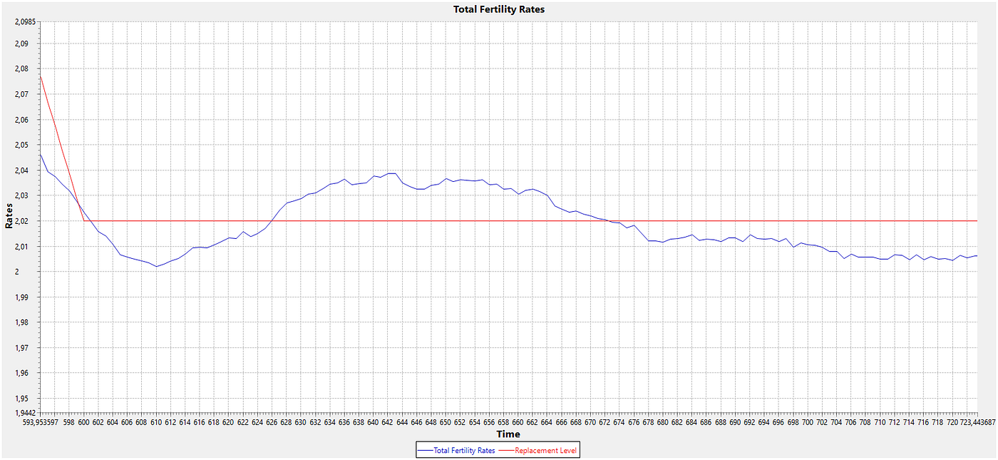
However, the development for total fertility rates is shifted: When population size goes above the eventual level and overshoots, the total fertility rate goes below the replacement level and vice versa. Basically, total fertility rates work against population size and stabilize it in this way. The oscillations are very slight if you look at the scale, with an initial amplitude of only about 0.02.

— — —

I find these results very encouraging because they reproduce actual developments quite well, at least qualitatively and I am not aiming for more here. As for actual life expectancies for Germany, the development was this (on the horizontal axis you have year minus 1,000, so 800 corresponds to the year 1800):

The development was somewhat longer than over a century, but roughly linear, except for dents resulting from the two World Wars. And we also have a broadly similar development for total fertility rates as in the simulation (on the horizontal axis again year minus 1000):

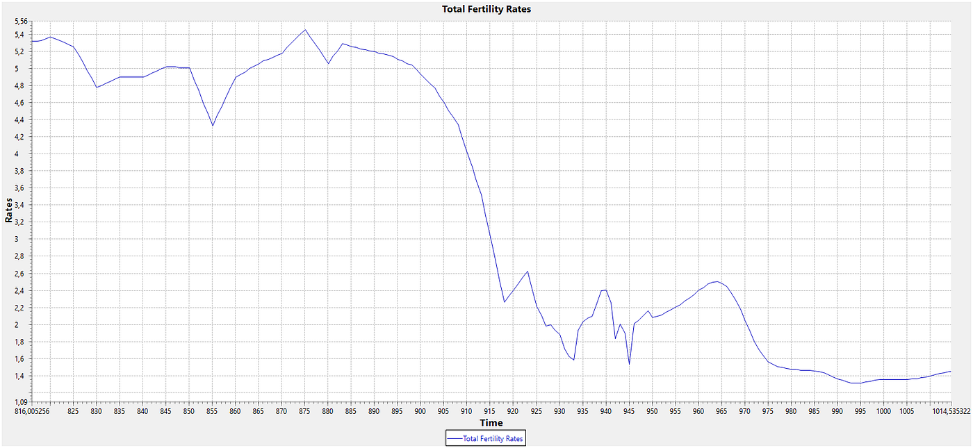
Total fertility rates remained at a high level mostly around 5 until well into the second half of the 19th century. Note that this was higher than the replacement level. In my scenario I assume a stable population at the start of the mortality transition to isolate its effect. In reality, the German population grew at a rather fast pace (see below). Total fertility rates peaked in the 1870s and then started to fall slowly until the end of the century. Already before World War I, the decrease becomes faster and continues afterwards, though with some back and forth. This is not entirely parallel with the results in my simulations. Obviously, more things are going here than only the mortality transition.

Nonetheless, my simple model yields a pretty good qualitative prediction that fertility will fall as a result of falling mortality. The sharp decrease of fertility from later in the 19th century on already puzzled observers at the time and has resulted in many explanations ever since that look for some major change in society. But in my model, the secular fall for mortality explains the decrease alone. Of course, also other things should have played a role in reality, eg. they could have affected the exact timing. It still seems as if their effect was rather modest and more about modifying the general development than driving it.

If you approach the situation from a Malthusian perspective, especially Malthus’ original theory, the whole development must be completely unexpected. The Malthusian assumption is that fertility stubbornly remains at a high level or even close to a maximum. As you can see that cannot be true for several reasons. Fertility before the demographic transition was well below a maximum, only sometimes above 5, not above 8 as has sometimes been observed for populations or even higher which seems possible. Total fertility rates even in the 19th century were actually much closer to a replacement level around 4 than to a maximum.

But if a population can pursue a level for total fertility rates that is considerably lower, by 3 or even more than the maximum, than where Malthusians think it always has to be, you have to concede that such a population has some control over its fertility, however they achieved that. It is by no means clear why a further decrease by perhaps 1.5 would be out of reach that would lead to fertility also around the replacement level. This alone could make it possible to stabilize the size of a population without any input from rising mortality.

From a Malthusian angle, when mortality fell to unprecedented levels, population growth should have sped up with fertility at a fixed level. The gap between new children that are born and those that die becomes larger. Instead population growth even slowed down in reality as you can see in the following graph for population sizes (horizontal axis again as year minus 1000, vertical axis in thousands, the dents correspond to the two World Wars):

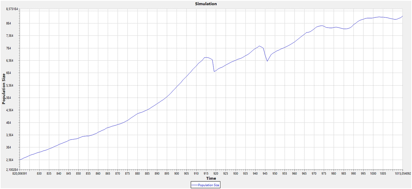
The population of Germany has kept growing over time even with below replacement fertility for half a century now. But that is to a large extent due to immigration, which I don’t capture in my simulation. However, neither do I account for emigration during the 19th century that had the effect that the number of people of German descent worldwide is somewhat lower, but in the same ballpark as the number of people in Germany.

— — —

The parallel development of a mortality transition and a demographic transition for fertility might be accidental and caused by other factors. However, it occurred also elsewhere. Here is the development for the UK, first for life expectancy where I have data back to the 16th century (data points are sparse and are linearly interpolated for earlier times, again years minus 1000 on the horizontal axis):

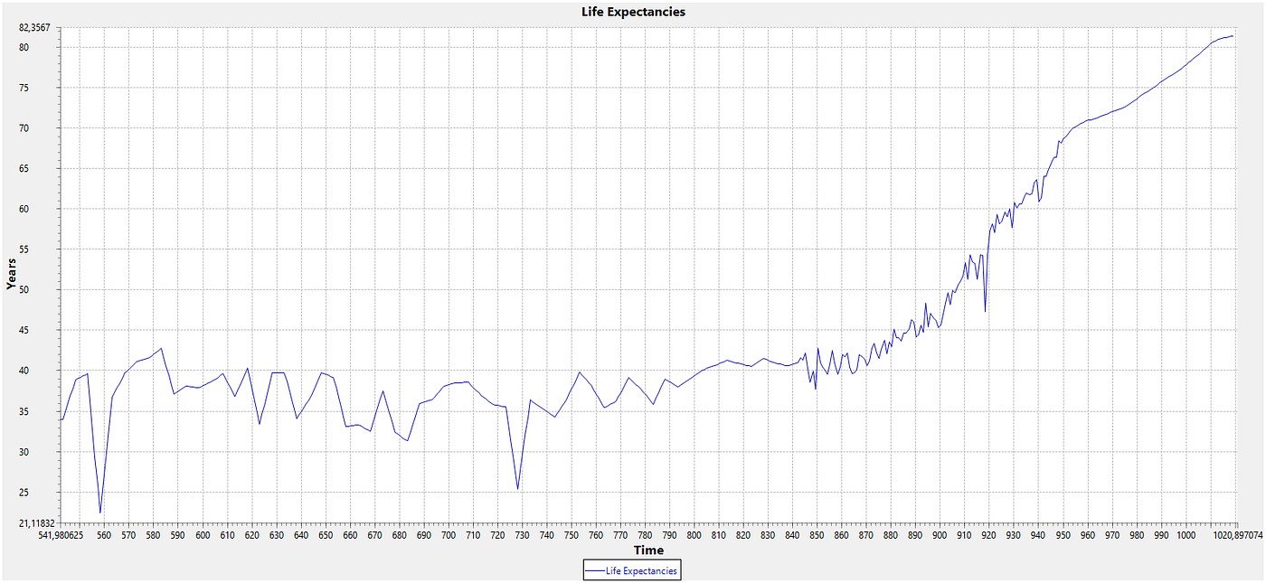
Life expectancy was roughly stable until the 18th century, though with a lot of short-term variation. It was actually already somewhat higher than for Germany in the decade from 1870 to 1880, mostly in the upper 30s. Then it begins to rise slowly to above 40 years in the early 19th century where it stays until about the 1870s. That’s when the development speeds up markedly and with less perturbation by the World Wars than for Germany. And again total fertility rates show the qualitative pattern that is expected in my model. As life expectancy starts to rise sharply, ie. mortality goes down, the demographic transition gets going around 1870:

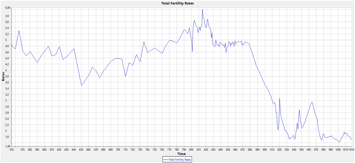
In the case of the UK, the development fits the predictions from the model even better than for Germany, with an almost linear decrease for fertility parallel with falling mortality and rising life expectancy, only somewhat interrupted by World War I. A speculative explanation for the smoother and more sluggish development in Germany might be that the UK was perhaps more homogenous, so developments in different parts occurred more in parallel, while you had an overlay of differently-timed developments in Germany. I don’t know whether that was so, but it seems at least plausible to me as the UK was more advanced than Germany and large parts of Germany took longer to develop.

You can again see that fertility also for the UK was never at the high levels Malthus assumes, close to a maximum that is possible, Instead they never went beyond slightly more than 6, but mostly remained in a similar range as for Germany before the demographic transition. Total fertility rates even went down to below the replacement level in the 17th century as population growth stopped for some time. Here it is clearly visible that the replacement level was actually in reach also for pre-modern populations. (I am skeptical about the accuracy of the earlier data, levels for total fertility rates appear too high to explain the actual development because they imply population growth that is too fast.)

As a final example now the classical country for a demographic transition: France. The country experienced a demographic transition already from the early 19th century on. Here are first the life expectancies for France:

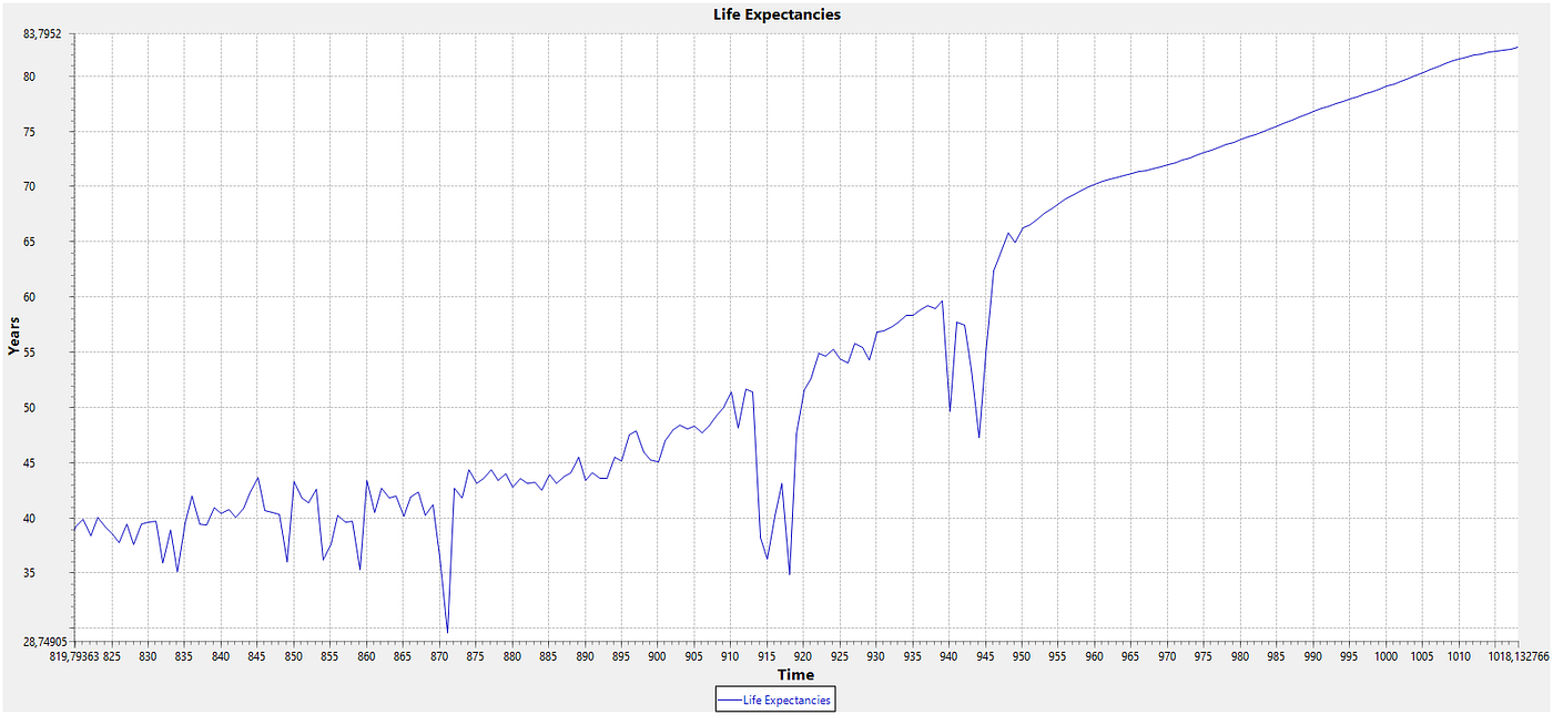
What is notable is that life expectancy was already around 40 years in about 1820, five years higher than for Germany half a century later. The improvement also started much earlier. In about 1870, life expectancy in France had risen to almost 45 years, about eight years higher than for Germany. The dents here are for the three wars that France suffered from: the war with Germany in 1870/1871 and the two World Wars. The development for total fertility rates is again parallel and consistent with the prediction from my model:

Total fertility rates are already comparably low in about 1800 with only 4.4. They then keep falling over the 19th century, a development that baffled those in France and in other countries at the time that had not yet experienced a demographic transition. For example, commentators in Germany in the 1870s ridiculed the “two-child system” in France and drew the conclusion that France was doomed because Germany would have continuing population growth at the then high levels. Ironically, the gloating about an inevitable demise for France came almost exactly at the time when the same development got going in Germany. And if my model captures the main driver correctly, those commentators were actually priding themselves on appallingly low life expectancies, at base: high child mortality, in Germany.

— — —

I will immediately grant that all this is not conclusive in favor of the above model, which I view only as a proof-of-concept. There must be more to actual developments than only the mortality transition and a parallel decline in ferility that it induces: Population increased by far more than than the 18% that I derive. But then the explanatory value for when demographic transitions start and how they develop is at least qualitatively in line with the data. Note though that this only works well for the early demographic transitions. Later demographic transitions did not started when life expectancy increased into the 40s and beyond, but often only when life expectancy was already pretty high.

Both observations do not refute such a model, though. As noted above, I keep the constant R’ fixed which I assume stands for something like a “level of distress” that may include many other things. It is such a “level of distress” only starts falling when life expectancy is high. You can live long, but still be abjectly poor. As I will demonstrate in further posts, you can obtain massive increases for population if you play around with this constant as a variable that rises for the most part independently from mortality. You then also get oscillation around a higher level once this development comes to a halt.

It is entirely possible that for other countries, there was a disconnect between population growth from rising reference levels driven by a “level of distress” and from falling mortality unlike in the case of European countries where it might have occurred in tandem. If so, massive population growth might just swamp the effect from falling mortality for some time. To a certain degree that was also the case in European countries where general population growth pulled fertility higher than in my simulation. It did not go below the replacement level as fast as I find.

What speaks for my model is that it is extremely parsimonious as it does not require a host of explanatory variables that are specific to certain times and societies. When mortality goes down, so does fertility. There is also no necessity to claim a miraculous turn of events in the 19th century that Malthusians are bound to resort to when they have to fix their theory. Human nature suddenly changed in 1800 or maybe 1870! Instead a theory in the vein of my theory can in principle handle all cases at all times in one go.

There is also another piece of evidence that can serve as confirmation. If you work through the connection between mortality and population size, you see that mortality goes down with population size, not up as Malthusians predict. But by construction, the causation cannot be that higher population size drives mortality down. Mortality is independent from it. Causation can only work the other way around: Falling mortality drives population size up.

Gregory Clark set out in his magnum opus “A Farewell to Alms” to show that population dynamics before 1800 or whatever were always Malthusian. He then brings a lot of data for England since the Middle Ages together to make his case. But ironically, when he runs mortality against population size, it is exactly the opposite from what he predicts: Mortality was lower for more population, higher for less population. Now I have no problem with this finding at all as it is fully in line with what my model predicts. For Gregory Clark, though, it is a huge problem as it is actually a complete refutation of his claim.

I love how he gets around this anyway. He has a graph where mortality goes down with population size so obviously that it is hard to deny. But then he just draws upward sloping lines through the downward sloping line that have no foundation in the data and calls those the values for different regimes. In those completely made-up regimes, he has the connection he wants to find. And then he just says that the downward-sloping line is a selection from the upward-sloping lines as the population runs through the regimes. If you allow this leap, you can, of course, prove practically anything you want. Down is up and up is down.

Even if the finding were that mortality sloped upwards in population size that would not refute my theory, only if the rise in mortality came from the food supply and so early that this is the binding constraint for population size. But falling mortality in population size refutes any Malthusian theory of population dynamics. There is always a case high up for populaton size where the food supply must become the binding constraint and mortality has to rise steeply. However, what falling mortality in size shows for an actual population is that it was regularly well below such a level and that a binding constraint from the food supply did not play a role. In other words: Gregory Clark has supplied the data to show that actual population dynamics, at least in the case of England in the Middle Ages, were non-Malthusian.