Null Hypothesis Significance Testing — Test for one Proportion

For students, novice researchers, and anyone who wants to brush up on their statistical knowledge.

This text discusses the general how and why of null hypothesis significance testing, with the specific topic of testing the fairness of a coin.

This article consists of four parts.

• Part 1. A Thought Experiment. Introducing Logic to Null Hypothesis Significance Testing with Simulations and Visualizations.
• Part 2. Behind The Thought Experiment. Statistical terminology and discussion of this thought experiment.
• Part 3. In Other Words. Translation of simulations into statistical formulas.
• Part 4. Let The Computer Do The Work. Application in a statistical tool.

Part 1. A Thought Experiment.

Introducing Logic to Null Hypothesis Significance Testing with Simulations and Visualizations.

There is a coin that is believed to be fair in probability, meaning that when you toss it, the probability of heads coming up is equal to the probability of tails coming up (probability of heads = probability of tails = 50%).

However, I think the coin is not fair and that heads has a greater chance than tails and I want to test that by tossing the coin 100 times.

I toss the coin 100 times and the outcome is 60 heads and 40 tails.

Based on this result, is the coin fair or biased?

The prediction came true with this outcome: heads came up more often than tails. But does this mean the coin is biased in favor of heads?

In order to make a statement about this, a statistical procedure is applied in which we want to find out how likely — in terms of probabilities — the outcome of 60 heads in 100 tosses is if the coin were actually fair, and on that basis make a statement about whether or not the coin in question is fair.

Step 1. Performing the test

As mentioned in the introduction, the test consists of tossing the coin whose fairness is in doubt 100 times, with the result being 60 heads and 40 tails.

Step 2: Constructing a probability distribution of the number of heads for 100 tosses of a fair coin.

What is the probability of zero heads in 100 tosses of a fair coin? What is the probability of one head in 100 tosses? And so on, up to what is the probability of 100 heads in 100 tosses? In this specific example, there are 101 possible outcomes.

This probability distribution provides a picture of all possible outcomes when the coin is fair. This provides a context for evaluating the specific outcome from step 1, 60 heads in 100 tosses.

There are several ways to create this probability distribution, one of which is to toss a fair coin 100 times in an infinite number of times, count the number of heads for each series, and then create a frequency distribution over the heads.

I let the computer do that, not endlessly, but often, 1,000,000 times.

And for each set of 100 throws, I don’t calculate the number of heads, but the proportion of heads (= number of heads/number of throws). That doesn’t affect the result and is often more readable.

The key point is that this now concerns a ‘theoretical probability distribution’, while step 1 concerns a concretely performed test with a concrete result.

Here are some examples of 100 coin tosses to give you an idea of what that looks like. If heads come up, give a 1, and if tails, give a 0.

100 throws per set:

0,1,0,0,0,1,0,0,1,0,0,1,1,0,1,0,0,0,1,0,1,0,1,1,0,1,1,0,1,1,0,0,1,0,0,0,0,1,0,1,0,0,1,0,1,1,1,0,0,1,1,0,0,0,0,0,0,1,0,1,0,0,1,0,0,0,0,0,1,0,1,1,1,0,1,0,0,0,0,0,0,0,0,1,0,1,1,0,0,0,0,0,0,0,0,1,1,1,1,0

1,0,1,0,1,0,0,1,1,0,1,1,0,1,1,0,0,0,1,0,0,1,1,0,0,0,0,0,1,1,1,1,0,1,0,1,0,0,1,1,1,0,0,1,0,1,0,1,1,1,1,1,1,1,0,1,0,1,0,1,1,0,1,1,0,1,1,1,0,1,1,0,0,0,0,0,1,1,0,1,1,0,0,1,1,1,0,1,0,1,0,0,1,0,1,1,0,1,0,1

1,1,0,0,0,1,0,0,1,0,1,0,1,0,0,1,0,1,1,1,0,1,1,1,0,1,0,0,1,1,0,0,0,1,0,0,1,0,0,0,1,0,1,1,0,1,0,1,1,0,1,0,1,1,0,1,0,1,0,1,0,1,1,1,0,1,1,0,1,0,0,0,0,0,0,1,1,1,0,0,0,0,1,1,1,1,0,0,0,1,0,1,1,1,0,1,1,0,0,1

and so on, up to 1,000,000 such sets. The proportion of heads of each set is then calculated.

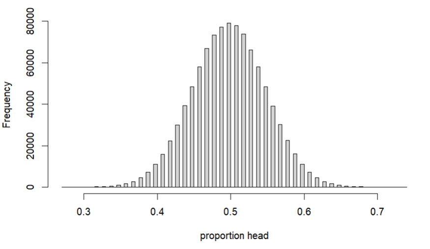
Below is the total result of the 1,000,000 proportions in what is called a histogram. A histogram is a graphical representation of a frequency distribution of numerical data. It shows the number of values ​​within certain (fixed) intervals, thus providing insight into the data’s distribution.

The proportion of the head is on the x-axis and the number of observations is on the y-axis.

Figure 1. Distribution of 1,000,000 sampled proportions.

Brief explanation of the apparent shape of the distribution:

Each time the coin is tossed, chance determines the outcome. With 100 fair coin tosses, a 50–50 outcome is most likely, and the further away from this 50–50, the smaller the chance.

The peak of the distribution is therefore a proportion of 0.5. The probability of a proportion of .0 — so 100 times tails or a proportion of 1.0 — so 100 times heads — is extremely small and actually not visible in the graph.

The distribution also has a clear bell shape, and the importance of this specific shape will become more clear again when discussing statistical formulas.

For my own convenience and visual appeal, I’ve made the frequency distribution a density. A density is a kind of smoothed histogram. The area under the curve is typically 1 (or 100%). It’s an approximation, not a completely accurate representation of reality here, but I don’t mind that so much; it’s the idea that counts here. And I’ll stop mentioning the x-axis, because that’s the proportion of head for the rest of this text.

Figure 2. Density plot of the distribution of 1,000,000 sampled proportions.

Step 3. Identify a given percentage of the observations furthest from the expected proportion head (0.5); in the “tails” of this probability distribution.

For example, 5% of all observations, distributed over the left and right tails each 2.5%, the red areas in the figure below.

Figure 3. 5% of the observations furthest from the expected proportion head, located in both tails.

Or 5% only in the right tail of the distribution.

Figure 4. 5% of the observations furthest from the expected proportion head, only in the right tail.

What is the logic of identifying these regions in the tail(s) of this distribution?

Before conducting the test, I agreed with myself that if the test result fell within this red area, relatively far from the expected value in the middle, I would consider this as striking and, for me, an indication that the coin is biased.

Step 4. Where does the result of the performed test fall in the constructed probability distribution?

As stated at the beginning, the result of the test is 60 heads and 40 tails, so the proportion of heads shown by the test is 0.6.

Because I expected beforehand that the probability of a head would be higher, I look at where this outcome falls in the last visualization, the variant with 5% of the most extreme observations in the right tail (Figure 4).

We can already see it a little bit, this falls into the red area.

I’ve colored the area from 0.6 to 1.0 blue to clarify this. The percentage of observations in this blue area is easy to calculate. 2.8% of all observations in figure 5 fall within the blue area.

Figure 5. The area from 0.6 to the right.

Now, what do I do with this outcome?

Now that the outcome (60 heads in 100 tosses) falls within the red range, I consider this result striking and an indication that the coin is biased.

But is the coin biased? We don’t know, we never actually know, that is, in the sense that it’s proven; we also don’t know (therefore) whether it’s fair.

But we have shown something, namely that the 0.6 heads proportion that has been found is “remarkably” far removed from the 0.5 proportion expected for a fair coin.

Time to put the above into a more formal statistical form and discuss it further.

Part 2. Behind The Thought Experiment.

Statistical terminology and discussion of this thought experiment.

What steps have been taken so far?

1. A coin whose fairness is in doubt is tested by tossing it 100 times. The result of the test is a heads ratio of 0.6.

2. A probability distribution has been made of the proportion of heads for 100 fair coin tosses.

3. A given percentage of the observations furthest from the expected proportion of heads in the “right tail” of this distribution has been identified.

4. The test result of 0.6 is placed in the probability distribution of a fair coin and a statement is made about whether or not the coin is biased.

These four steps together form a test for a proportion.

I would like to link more formal terminology to these 4 steps and explain them in more depth.

ad 1. A coin whose fairness is in doubt is tested by tossing it 100 times. The result of the test is a heads ratio of 0.6.

Tossing the numbers 100 times is a random sample. A random sample is a selection from a larger group, the population. Sample size (here 100) is denoted by the letter “n,” so n = 100.

A proportion is a statistic. A statistic is a value that describes a sample. A parameter is a value that describes a population. A statistic is an estimator of a parameter.

ad 2. A probability distribution has been made of the proportion of heads for 100 fair coin tosses.

The probability distribution of the proportion of heads when tossing a coin 100 times is called a “sampling distribution” or, more specifically, a sampling distribution of a statistic.

Specifically in this example, we are considering the sampling distribution of the proportion heads of a fair coin tossed 100 times.

The technique used to create this sampling distribution is called ‘bootstrapping’.

Bootstrapping involves taking a random sample with replacement (see below what that means) from an existing sample a large number of times, equal to the size of the existing sample, and calculating a statistic (in this case a proportion) on it each time.

In our example, you could imagine a sample of 50 heads and 50 tails (expectation of a fair coin), or fifty 1s and fifty 0s. For example:

1,1,1,1,1,1,1,1,1,1,1,1,1,1,1,1,1,1,1,1,1,1,1,1,1,1,1,1,1,1,1,1,1,1,1,1,1,1,1,1,1,1,1,1,1,1,1,1,1,1,0,0,0,0,0,0,0,0,0,0,0,0,0,0,0,0,0,0,0,0,0,0,0,0,0,0,0,0,0,0,0,0,0,0,0,0,0,0,0,0,0,0,0,0,0,0,0,0,0,0

From those 100 digits, I randomly select one and record it. I don’t remove it from the set of 100 digits (hence the term, “with replacement”) and I randomly select again a digit, and so on, until I have 100 observations. Technically, this is the same as selecting a number 100 times from an infinite population of numbers with the value 0 or 1, where 0 and 1 occur equally, and the same as tossing a fair coin 100 times. And then I calculate the head proportion from that.

That process was repeated 1,000,000 times to create the sampling distribution.

This simulates what statisticians are interested in: the distribution of a statistic when a sample is drawn an infinite number of times from an infinite population.

1,000,000 is not infinity and therefore an approximation of the result of sampling infinitely.

ad 3. A given percentage of the observations furthest from the expected proportion of heads in the “right tail” of this distribution has been identified.

The 5% most extreme observations in the right tail of the probability distribution are called the significance region, or rejection region. I only look at the right tail because I think heads are more likely. This is called one-tailed testing (right-tailed in this case).

If I suspected the coin was not fair, but had no idea whether heads or tails would have a higher probability, I would look at both tails (5% divided between the left and right tails, 2.5% each): two-tailed testing.

While the red region in Figures 3, 4 and 5, the 5% most extreme observations, is called the significance region, the number 5 itself is called alpha (usually represented as α) and is noted as α = .05 or 5%.

Alpha is a value chosen by the researcher. 5% is a common choice, especially in the social sciences. There’s more to be said and nuanced about this. More on that later.

ad 4. The test result of 0.6 is placed in the probability distribution of a fair coin and a statement is made about whether or not the coin is biased.

Before conducting the test, I decided that if the test result falls within the 5% most extreme observations in the right tail of the probability distribution, I would consider that striking and an indication that the coin is biased.

“Striking” and “indicative that the coin is biased” are called “statistically significant”.

It’s important to remember that the sampling distribution applies to a fair coin. A significant result therefore means a striking result for a fair coin.

The blue area in Figure 5, the area in the distribution from 0.6 onwards, is called the p-value (noted as p; in our test we would write “p = .028”) and is the probability of the test result (0.6) found, or an even larger proportion , so the blue area under the curve in figure 5, between 0.6 and 1.0.

Formal description in terms of “hypotheses”:

The assumption that the coin is fair is called the null hypothesis: H0.

Formal notation. H0: probability of heads = .5. Or, P(heads) = .5

The assumption that the coin is not fair, specifically that the probability of heads is greater, is called the alternative hypothesis: H1.

Formal notation. H1: Probability of heads > .5. Or, P(heads) > .5

Then after the test:

If the p-value is less than or equal to alpha, we “reject the null hypothesis.”

If the p-value is greater than alpha, we “do not reject the null hypothesis.”

What does “reject (or not reject) the null hypothesis” actually mean?

First of all, what doesn’t it mean?

Rejecting the null hypothesis does not mean that H0 is not true, it does not mean that H1 is true, nor does it say anything about the probability that H0 is true or that H1 is true.

Failure to reject the null hypothesis does not mean that H0 is true, it does not mean that H1 is not true, nor does it say anything about the probability that H0 is true or that H1 is true.

What then does rejecting the null hypothesis mean?

What it means if we reject the null hypothesis is essentially as stated before: the outcome is striking and is an indication that H1 is true.

Scientifically speaking, this means that, based on the test, we assume for now (we provisionally assume) that H1 is true; in other words, we “act as if” H1 were true (until possible new tests indicate otherwise).

Or even more cautiously: the test result supports H1.

What if the null hypothesis is not rejected?

Then the test result does not support H1.

To summarize the coin example: the test outcome is statistically significant because the p-value is smaller than the predetermined alpha.

In a scientific article, something like the following will be written (alongside a full description of the test and the results): The outcome of the test is significant at an alpha of 5% (p = .028).

Figure 6 provides a schematic illustration of the sampling distribution, p-value and alpha based on Figure 5.

Figure 6. Schematic illustration of the sampling distribution, p-value and alpha.

(The sampling distribution actually runs from 0 to 1 from the beginning of the left tail to the end of the right tail, and the p-value and alpha run to 1. I mainly hope the picture clarifies which areas are involved.)

The test is ready.

There are two important additional questions that need to be answered.

Was n = 100 a wise choice?

Was α = 0.05 a wise choice?

The answer to both questions is no, that is, the choices are not sensible in the sense that no justification has been given for them.

How can an account be given for n and alpha?

Alpha is an area in the tail(s) of the sampling distribution under H0, hence belonging to H0 and is the probability that we reject H0, when H0 is true.

It’s an incorrect decision to reject H0 when H0 is true, but it can and will happen by chance (namely alpha). The correct decision would be not to reject H0.

This is the “tension” or “calculated risk” that is used in null hypothesis significance testing.

Rejecting H0 when H0 is true is called an “type I error” (= α).

By definition, a type I error can only occur if H0 is true.

Alpha is determined by the researcher himself.

Just as H0 can be rejected when H0 is true, the sample result can also fall outside the significance region while H0 is not true.

Not rejecting H0 when H0 is not true is also an incorrect decision; the correct decision would be to reject H0.

Failing to reject H0 when H0 is false is called a “type II error”; H0 is then “falsely not rejected.” The probability of this error is called beta (ϐ).

By definition, a type II error can only occur if H1 is true.

The probability of rejecting H0 when H0 is false is the complement of beta: 1 — beta. This is called “power”: the probability of correctly rejecting H0.

Beta, and therefore power, can only be calculated if H1 is known. A specific H1 must be formulated for this.

An example:

Suppose that — before any testing has even taken place — I would consider a 5% deviation from the coin in the example above to be very important and want to have a certain certainty (say 80% chance) of finding this effect (the deviation from H0) as statistically significant in a test.

In addition to the sampling distribution under H0: P(head) = .50, I create a second sampling distribution, namely under H1: P(head) = .55.

From the combination of both I can deduce how often an assumed real effect will also emerge as significant from a test.

Figure 7 shows the sampling distribution of the proportion of heads with n = 100 and P(head) = .50 (same as Figure 2).

Figure 7. Sampling distribution under H0.

A sampling distribution of the proportion of heads with n = 100 and P(head) = .55 is also created using bootstrapping and added in Figure 8.

Figure 8. Adding the sampling distribution under H1.

In Figure 9, the significance region is added to the right tail of the sampling distribution under H0 (alpha = .05).

Figure 9. Alpha.

The significance area starts at .58.

This means that all sample test results with a value of .58 or greater will be considered statistically significant.

In this second thought experiment, assuming H1 is true and assigning H1 a precise value, we can now calculate the probability that the test (100 coin flips) will yield a proportion less than .58. It is the area in the sampling distribution under H1 left of .58: the grey area in Figure 10. This is beta.

Figure 10. Beta.

The blue area in Figure 11 is all outcomes greater than or equal to .58 under H1: 1 — beta or power.

Figure 11. 1 — beta.

The relative area of the blue region in the sampling distribution under H1 is .31 and of the grey region is .69, totaling 1.0.

This means that if H1 is true with P(head) = .55, then with a sample size of n = 100 and an alpha of .05, there is a 31% a theoretically deduced chance that this will come out statistically significant from a test.

The left grey area represents beta, or the probability that the null hypothesis will be wrongly not rejected; wrongly because H1 is assumed to be true.

The blue right region represents the probability that H0 will be correctly rejected: 1- beta, power: the probability to correctly reject H0.

The power of this test is therefore 31%, so based on H1 it has a 31% chance of “success” in what it is intended to do, namely make it plausible that the coin is not fair.

A test with a power of 31% is not or hardly informative; there is little point in performing this test because it has little potential to detect the assumed effect as significant.

What is an acceptable power level? A power level of 80% is often cited as acceptable in the social sciences.

How do we get a test with 80% power? That can be acheived either by increasing the sample size, or by increasing alpha.

Increasing alpha will increase the region of significance, the region will start at a smaller proportion on the x-axis, and therefore making beta smaller, and therefore increasing the power.

If I were to insist on a power of .80 in the current example, with n = 100 an alpha of almost .4 would have to be chosen.

Figure 12. sampling distribution with higher alpha.

The achieved power is .82, not exactly the target of .80, but it’s the thought that counts.

An alpha of .4 also produces a test with little information value: if H0 is true, H0 is rejected in 40% of all tests.

Any other compromise can be sought between alpha and beta, between type I error and type II error.

The question here is how ‘bad’ it is to wrongly reject H0 versus how ‘bad’ it is to wrongly not reject H0. In the first case we confirm an effect that does not actually exist, in the second case we deny an effect that does actually exist. The impact of a type I error or a type II error is context-dependent. For example, the significance of a wrong decision in a medical examination differs from the referee’s toss that determines who starts the match first.

If an acceptable compromise between alpha and beta cannot be found, it is actually better to forgo the test altogether.

Another simple solution to obtain greater power is to choose a larger sample size.

In general, a larger sample is more reliable than a smaller sample.

Or rather, a larger sample has a narrower sampling distribution than a smaller sample from the same population, that is, more centered around the peak of the distribution.

There is a precise relationship between sample size and the dispersion of the sampling distribution.

I will demonstrate this with the following three sampling distributions, with sample sizes of 100, 400, and 1.6, respectively.

Figure 13. the sampling distribution at n = 100 and P(head) = .5.

If we look at the 90% of observations around .5, we see that it lies between .42 and .58.

If we make the sample 4 times larger, so n = 400 and P(head) = .5, then this is the sampling distribution.

Figure 14. the sampling distribution at n = 400 and P(head) = .5.

90% of the observations around .5 fall between .46 and .54.

The sample size is 4 times as large, and the 90% interval has gone from .58 — .42 = .16 to .54 — .46 = .08, so it has become 2 times smaller.

For a 16 times larger sample, so n = 1,600 and P(head) = .5, the 90% interval is between .48 and .52.

Figure 15. the sampling distribution at n = 1,600 and P(head) = .5.

With a 16 times larger sample size, the 90% interval has become 4 times smaller (.52 — .48 = .04).

The general rule as it appears here is: as a sample size becomes x times larger, the spread of the sampling distribution (defined here as the 90% interval around the expected value) becomes square root (x) times smaller.

How large should the sample be to have a power of 80% with an alpha of 5% and H0: P(head) = .50 and H1: P(head) = .55?

With a bit of trial and error I arrived at n = 600.

Figure 16: the power at n = 600.

The achieved power is now .81, not exactly the target .80, but again, it’s the thought that counts.

In summary, if we want to test a coin for fairness and we want to have an 80% chance of finding a 5% deviation in a one-tailed test with an alpha of .05 as statistically significant, we need to toss the coin at least 600 times.

Was an alpha of .05 and a power of .8 the best choice? That’s up to the researcher and depends on the context.

Sample size is often the bottleneck. Flipping a coin 600 times isn’t a big problem, but finding 600 patients to test a new drug can be, to give an example from research practice.

The conclusion is that simply determining alpha and choosing a sample size is not wise, but is better done in the context of a power analysis.

Wrapping up:

Using bootstrapping, sampling distributions of a proportion were constructed.

The sampling distribution is central to statistical testing and power analysis.

Bootstrapping literally produces what is important in statistics: the probability distribution of a statistic when a test is repeated endlessly.

Part 3. In Other Words.

Translation of simulations into statistical formulas.

In practice, bootstrapping will not be used very often, but mathematical formulas that deliver quite the same result will be used.

The sampling distributions presented thus far have been notable for their distinctive bell shape. This shape is commonly known as a “normal distribution.”

A normal distribution is a symmetric distribution with a given mean and a given standard deviation with general and known properties.

A standard deviation is a measure of dispersion in a distribution, the spread around the mean. Think of it as a kind of average distance of all data points from the center of the distribution.

For a heads-tails, yes-no, success-failure, 0–1 variable, also called a binary variable, the standard deviation is:

p = proportion. So a data set with 50 heads and 50 tails has a standard deviation of the square root of .5 * .5 = square root of .25 = .5.

In itself this standard deviation doesn’t tell me much, what is more telling is the standard deviation of the sampling distribution:

The standard deviation of the sampling distribution is called the standard error, or SE.

So the standard deviation is a measure of dispersion for a sample and the standard error is a measure of dispersion for a sampling distribution of a sample statistic. It is important to keep these two conceptually distinct.

The standard error of the sampling distribution of the proportion of heads for 100 fair coin tosses is the square root of (.5 * .5 /100) = square root of .0025 = .05.

A normal distribution allows statements to be made about the number of observations, or the area of a density, that falls between two different values on the x-axis.

For example, between the mean minus one standard deviation and the mean plus one standard deviation, in a normal distribution we typically find 68.2% of all observations.

In a normal distribution, we find 95.4% of all observations between the mean minus two standard deviations and the mean plus two standard deviations.

In a normal distribution, we find 99.7% of all observations between the mean minus three standard deviations and the mean plus three standard deviations.

The sampling distribution for a proportion is normally distributed. That is, an assumption must be made about the number of observations: a rule of thumb is that both n p and n (1-p) should be greater than 5. If there are too few observations, the actual sampling distribution will no longer neatly follow the normal distribution.

In our example, n p = 100 .5 = 50 and ditto for n * (1-p), so the sample size satisfies the rule of thumb.

Applied to the example of the sampling distribution of the proportion of heads after 100 fair coin tosses:

We find 68.2% of all observations between the mean (.5) minus one standard deviation (1 * .05) and the mean plus one standard deviation.

We find 95.4% of all observations between the mean (.5) minus two standard deviations (2 * .05) and the mean plus two standard deviations.

We find 99.7% of all observations between the mean (.5) minus three standard deviations (3 * .05) and the mean plus three standard deviations.

Figure 17. A normal distribution.

A normal distribution can be transformed into a standard normal distribution. A standard normal distribution is a normal distribution with a mean of 0 and a standard deviation of 1.

A standard normal distribution is also called a Z-distribution.

The transformation from a normal to a standard normal distribution actually occurs when applying the formula for the test for a proportion:

The Z value in our example is the difference between the test result (100 tosses) = .6 (the p-hat) and the expected result if the coin was fair = .5 (p with subscript 0) divided by the standard error under H0 (which we also calculated earlier).

If we want to get it absolutely right, we also apply a “continuity correction.” In Figure 1, we saw that the distribution is actually discrete, and with the Z distribution, we superimpose a continuous distribution on top of it.

This means that half of a bar (0.5/100) is incorrectly excluded. A small detail, but important, especially with smaller samples.

To clarify this, here is an example of that “half bar” based on a hypothetical discrete distribution.

A normal distribution is superimposed on this discrete distribution.

Figure 18. A hypothetical discrete distribution with a normal curve superimposed on it.

You can see that the normal distribution cuts roughly through the middle of the bars.

If we are interested in the area of ​​the six rightmost blue bars in Figure 19 and were to use the area under the normal curve for this, we would be missing the gray half-bar.

Hence the continuity correction.

Figure 19. What we would miss if we used the normal distribution without continuity correction (grey half-bar).

Z calculation with continuity correction:

The difference between the test outcome and the expected outcome under H0 is 1.9 standard deviations to the right of the center in the Z-distribution.

The probability of exceeding Z = 1.9 (= p-value) can be looked up in a Z-table, where it turns out to be 0.02872. You can probably find a Z-table at the back of your statistics textbook, or otherwise online, for example at https://en.wikipedia.org/wiki/Standard_normal_table.

This is close to the .02846 p-value found with bootstrapping.

Another test using a statistical formula is known as the Binomial test, in which the sampling distribution is calculated exactly using probability rules.

For reasons of time and space, I won’t discuss this test here, but you’ll likely encounter it in literature and analytical tools.

For the same reason I will also omit the formula(s) for power analysis and will demonstrate these in part 4 using a statistical tool.

Part 4. Let The Computer Do The Work.

Application in a statistical tool.

Statistical formulas are applied in the background in analytical tools, where p-values and power results are then output “automatically”.

There are several tools for performing statistical tests, including the open source and freely available tools R, Python, and JASP.

R and Python work on the basis of custom code, JASP works with a menu.

I would like to demonstrate the results using JASP (https://jasp-stats.org/).

JASP is a good choice for beginners and anyone who doesn’t need to write code as much. A wealth of support documents (https://jasp-stats.org/jasp-materials/) are available on the website.

The result of the test (60 heads and 40 tails) is read as a table with 1 column and 100 rows.

Small screenshot of a part of it (the first 10 rows):

Under “Frequencies,” JASP has a “Binomial Test” option and no Z-test, so we choose “Binomial Test,” a good choice anyway.

The column named “Head” goes to the “Variables” box on the left side of the menu. The Test value is .5, and under “Alt. Hypothesis,” “> Test value” is selected for a right-tailed test.

In the output on the right, you’ll see the p-value: 0.02844. This is even closer to the result of the bootstrap analysis than the Z-test. This is not surprising, as the Binomial Test is calculated precisely, and the bootstrap analysis (with extensive resampling) is essentially so as well.

A brief demonstration of power analysis as previously performed with bootstrapping.

In the Power tab, you can calculate a required sample size based on the expected effect (.55 versus .50), alpha, and power.

There’s a lot going on in this picture.

The “One Sample Proportion Test” is chosen for the test. We want to calculate the required sample size based on: H0: 0.50 H1: 0.55 Power: 0.8 Alpha: 0.05 The test is right-sided.

Result: the recommended n = 617. Using bootstrapping I earlier arrived at n = 600 for even slightly higher power, but I’m not dissatisfied with it.

JASP also provides a chart with sampling distributions under H0 and H1, as shown in the screenshot. And various additional outputs if desired.

The realized power can also be calculated here based on the chosen sample size, alpha, and expected effect.

A small note: the difference between 0.50 and 0.55 is converted in JASP to a standardized effect measure, “Cohen’s |h|”. Effect measures are quite a story in themselves, and I won’t go into them for now.

This concludes my discussion of the test for one proportion.

In subsequent articles, I will expand on this topic to:

• A test for the difference between two proportions.
• A test for the difference between two means.
• The regression approach to the test for the difference between two means.