MATHEMATICS EXPLAINED

The Hidden Geometry Of Space

How Manifolds Reveal The Shape Of Curved Worlds, Moving Systems, And Modern Data

The Earth does not feel round.

Stand on a road, look toward the horizon, and the world seems almost flat. Buildings rise vertically. Cars move along the ground as if the ground were a plane. A ball rolls on the pavement without giving any hint that it is moving on the surface of a sphere.

And yet the Earth is curved.

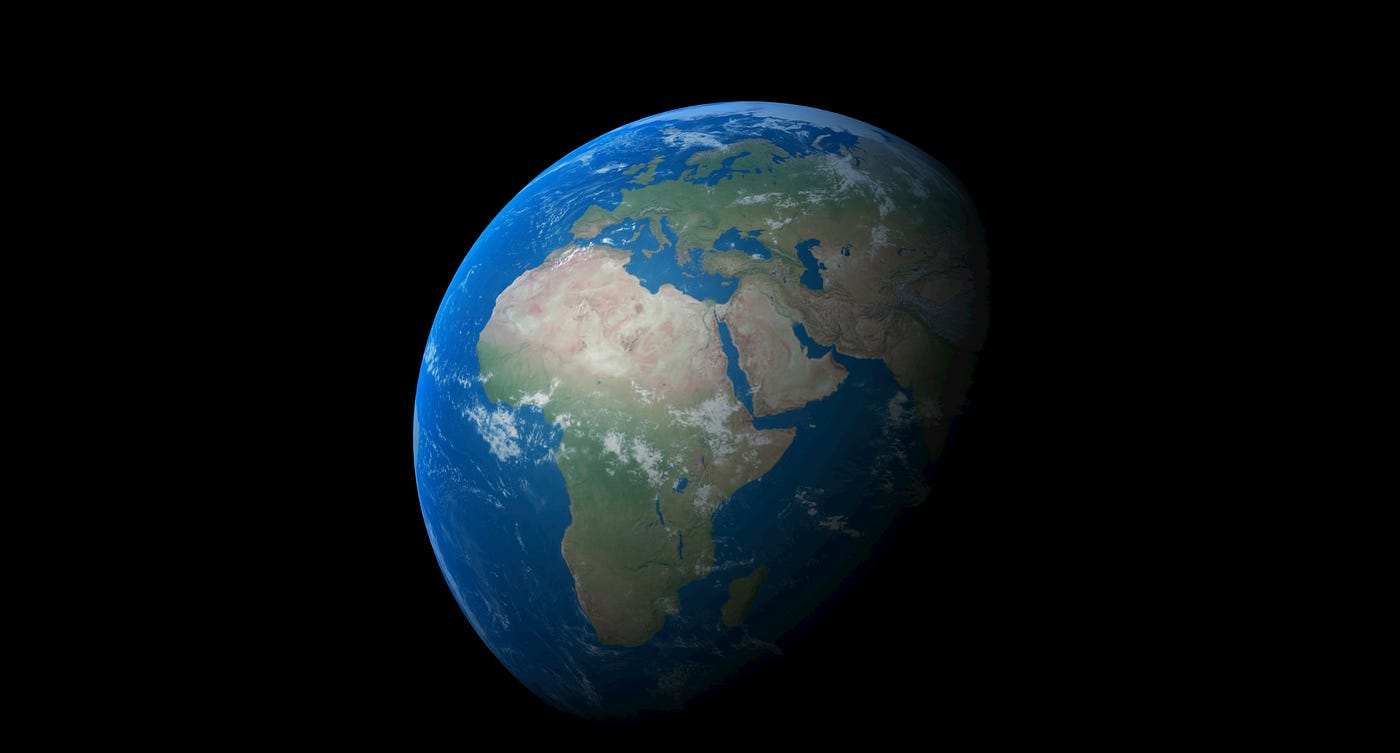
Earth seen from space, where the curvature hidden from everyday experience becomes unmistakable. Photo by colin km on Unsplash.

The problem is scale. A tiny part of a sphere can look almost flat, just as a tiny part of a circle can look almost straight.

This simple observation leads to one of the most powerful ideas in modern mathematics.

A space can look flat when we zoom in, even if it is curved, twisted, closed, or strange when we see it as a whole.

Mathematicians call such spaces manifolds.

A manifold is a space where every point has a small neighborhood that behaves like ordinary Euclidean space. A one-dimensional manifold looks locally like a short open interval. A two-dimensional manifold looks locally like a small open patch of the plane. Higher-dimensional manifolds follow the same idea, even when we cannot picture them directly.

Manifolds matter because they let us separate the coordinates we use from the hidden shape underneath: sometimes that shape carries curvature, sometimes it records possible motions, and sometimes it organizes high-dimensional data.

This tension, local simplicity and global mystery, changed geometry. It gave Einstein the mathematical language of curved space-time. Today, it appears in robotics, physics, artificial intelligence, and data science.

Manifolds are not just shapes. They are the hidden geometry of possible worlds.

The Shape That Looks Simple Up Close

Imagine a tiny ant walking on the surface of a very large ball.

The ant does not see the ball from the outside. It experiences only the small region around its feet. If the ball is large enough, that small region looks like a flat plane. The ant can move forward, turn left, turn right, and measure short distances. Locally, its world behaves like ordinary two-dimensional space.

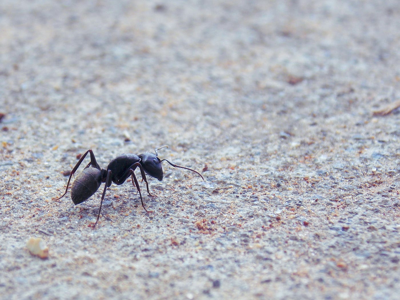
A tiny ant experiences only the small surface beneath its feet. On a sufficiently large curved world, that local patch can feel flat even when the whole surface is not. Photo by Jenny Chambers on Unsplash.

But the whole surface is not a plane. It is a sphere.

That is the basic idea of a two-dimensional manifold. Near every point, the surface looks like a piece of the plane. Globally, it may close on itself, curve, or have a more interesting structure.

A circle gives the one-dimensional version of the same idea. If we zoom in on a tiny part of a circle, it looks like a short straight line. An ant living on the circle would experience its local world as line-like. Only by walking far enough would it discover that the line closes back on itself.

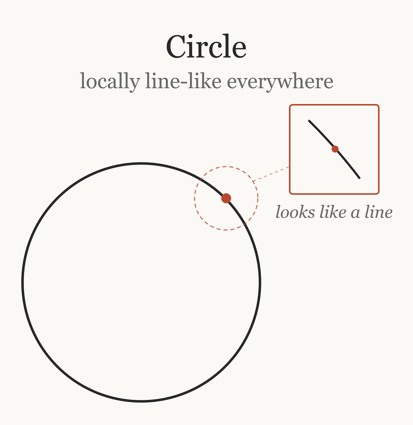
A circle is curved as a whole, but a tiny neighborhood around any point looks like a short line segment. This is the one-dimensional version of the manifold idea.

A torus, the surface of a doughnut, works similarly in two dimensions. Near any point, it looks like a small flat patch, even though the whole surface has a hole.

This is why manifolds are useful. The whole space does not have to be flat. It only has to behave like flat space when examined closely enough.

When The Local Test Fails

Not every shape passes the local test.

Take a circle. At every point on the circle, a tiny neighborhood looks like a line. Nothing unusual happens. The circle is a one-dimensional manifold.

Now consider a figure eight, made of two loops crossing at one point. Away from the crossing, everything looks line-like. But at the crossing itself, four branches meet. A small neighborhood around that point does not resemble a single line.

That one point breaks the manifold structure.

The figure eight is therefore not a manifold, at least not as a whole.

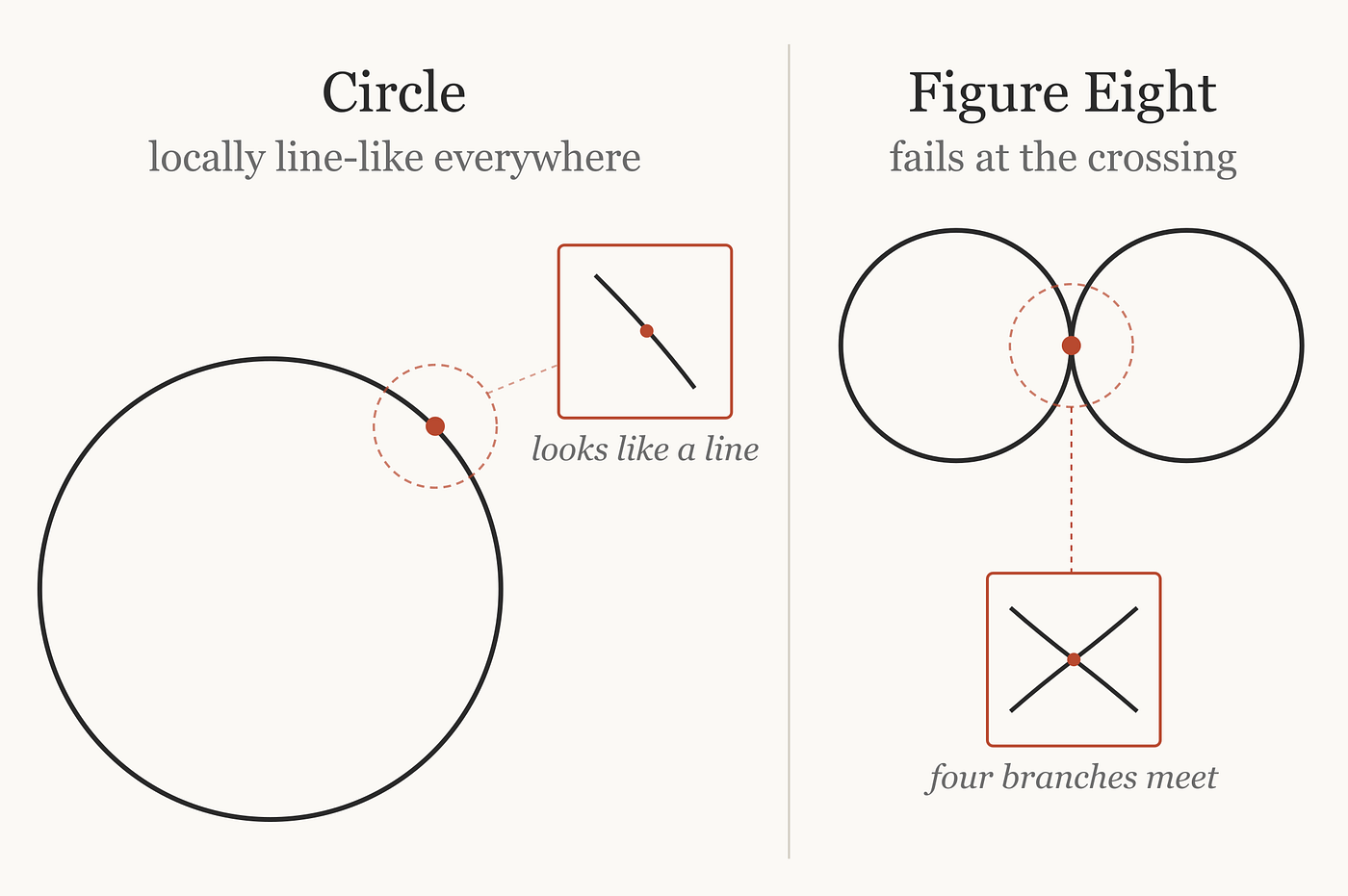
A circle is locally line-like at every point. A figure eight fails at the crossing, where the local neighborhood no longer resembles a single line.

Sharp points introduce a related but subtler issue.

A cone looks like a smooth surface almost everywhere. Its tip is special. If we cut the cone along one line from the tip to the base and unroll it, the cone becomes a flat sector. Something is missing: the angles around the tip do not add up to a full turn. For example, the unrolled sector might contain only 300 degrees around the tip instead of 360 degrees. The missing 60 degrees is the cone’s angle deficit.

This does not fail in exactly the same way as the figure eight. Topologically, the cone tip can still have a disk-like neighborhood. But geometrically, it is not an ordinary smooth point of a surface. The metric has a singularity there: curvature is concentrated at the tip.

This distinction matters. A manifold can be studied at different levels. A topological manifold only needs the right local shape. A smooth or Riemannian manifold also needs enough structure to support calculus, distances, angles, and curvature without singular points.

A Triangle With Three Right Angles

For thousands of years, geometry meant Euclidean geometry.

In Euclidean geometry, parallel lines do not meet. The shortest path between two points is a straight line. The angles of a triangle add up to 180 degrees.

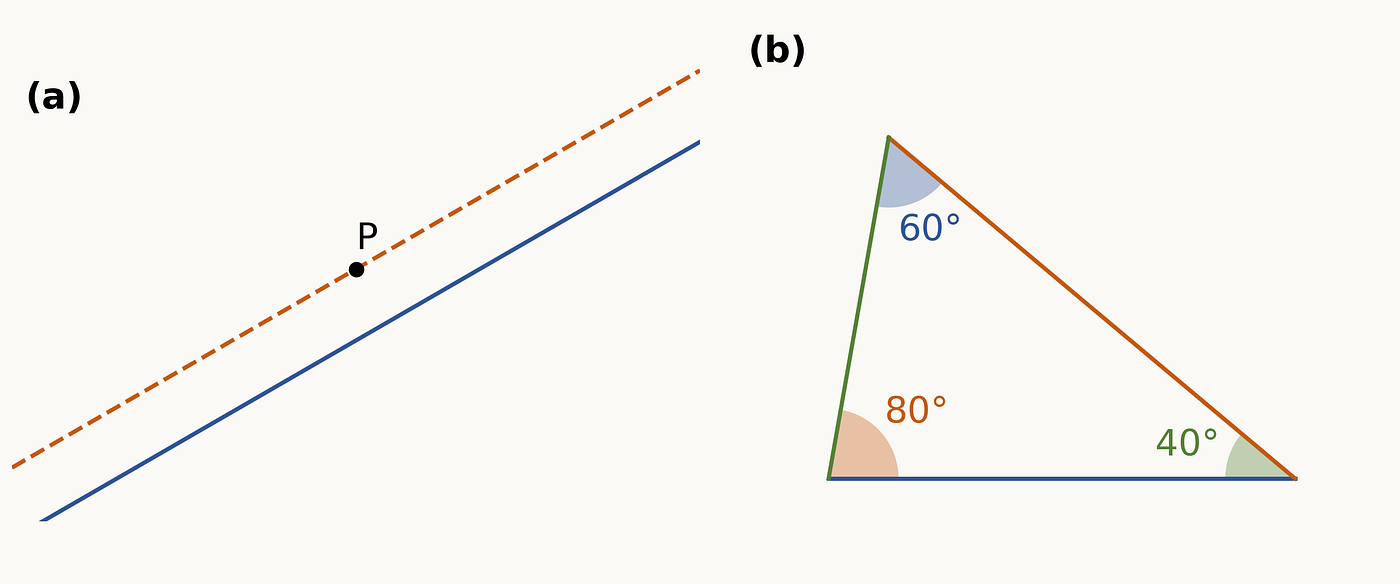
Two basic rules of Euclidean geometry: (a) parallel lines remain separated, and (b) the angles of a triangle add up to 180 degrees.

But on a curved surface, these familiar rules may fail.

The easiest way to feel this is to draw a triangle on a sphere.

Start at the North Pole. Travel south along one line of longitude until you reach the equator. Then move along the equator by 90 degrees. Finally, travel back to the North Pole along another line of longitude.

You have formed a triangle on the surface of the Earth.

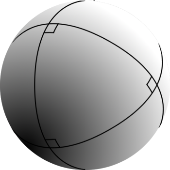
A triangle formed by two meridians and the equator can have three right angles, giving an angle sum of 270 degrees.

At the North Pole, the two lines of longitude meet at a right angle. At the first point on the equator, the meridian and the equator also meet at a right angle. At the second point on the equator, the same thing happens again.

The triangle has three right angles. Its angle sum is therefore 270 degrees. Not 180 degrees.

This example is small, but it changes everything. The rules of geometry depend on the space in which the geometry is taking place.

On a flat plane, triangles have 180 degrees.

On a sphere, triangles can have more, as the 270-degree triangle above shows.

On a saddle-shaped surface, or in hyperbolic geometry, triangles can have less than 180 degrees. In the limiting case of an ideal hyperbolic triangle, whose vertices lie on the boundary at infinity, all three angles are 0 degrees.

Geometry is not just about figures. It is about the space that contains them.

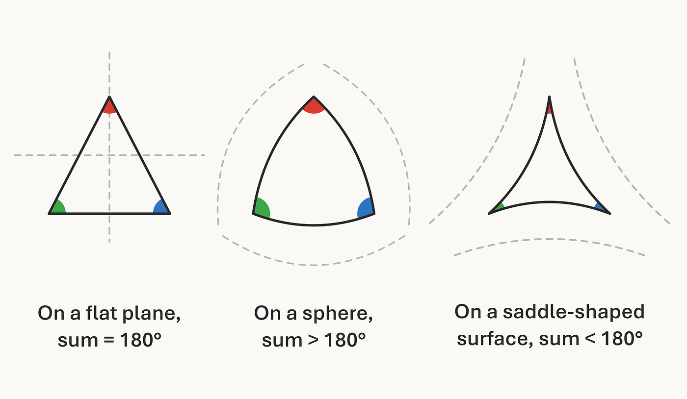
The angle sum of a triangle depends on the geometry of the surface. It is 180 degrees on a flat plane, greater than 180 degrees on a sphere, and less than 180 degrees on a saddle-shaped surface.

The Lecture That Changed The Meaning Of Space

In the middle of the 19th century, Bernhard Riemann pushed this idea much further.

Before Riemann, geometry was usually imagined as the study of shapes inside a larger space. A curve sits in a plane. A surface sits in three-dimensional space. A sphere is imagined as a ball in a room.

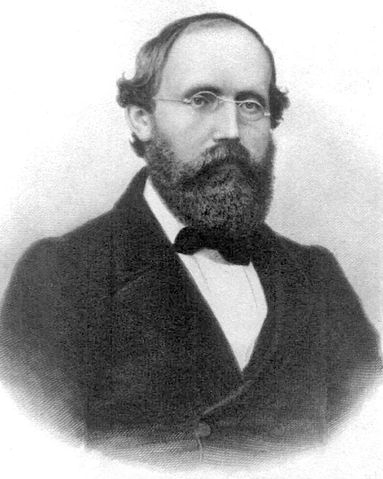
Bernhard Riemann (1826–1866). His 1854 Göttingen lecture changed the meaning of geometry by treating space itself as a mathematical object with its own internal structure. Image: Wikimedia Commons, public domain.

Riemann’s radical move was to ask whether a space could be studied from within.

A surface did not need to be understood only as something embedded in a larger surrounding world. It could have its own internal geometry. Distances, angles, and curvature could be properties of the space itself.

The scene was Göttingen, 1854. Riemann had to deliver a lecture for his Habilitation, the qualification needed for an academic teaching position. As was customary, he submitted three possible topics. He expected Carl Friedrich Gauss to choose one of the first two, which Riemann had prepared more carefully.

Gauss chose the third.

It was the most difficult one: On The Hypotheses Which Lie At The Foundations Of Geometry.

Riemann had only a short period of concentrated preparation for one of the deepest questions in mathematics, while also carrying the burden of other research work and fragile health. The result could easily have been a cautious academic exercise.

Instead, on June 10, 1854, Riemann stood before his audience in Göttingen and described a new way of thinking about space. Geometry, he suggested, did not have to begin with a fixed flat background. A space could have dimension, distance, and curvature from within.

Space was no longer merely the passive stage on which mathematics happened.

Space itself became the object of mathematics.

According to later accounts, Gauss was deeply impressed. He walked away from the lecture visibly moved and told Wilhelm Weber that Riemann’s work had exceeded his expectations.

But the world did not immediately change. Riemann died in 1866, at only 39, from tuberculosis. His lecture was published two years later, after his death, by Richard Dedekind.

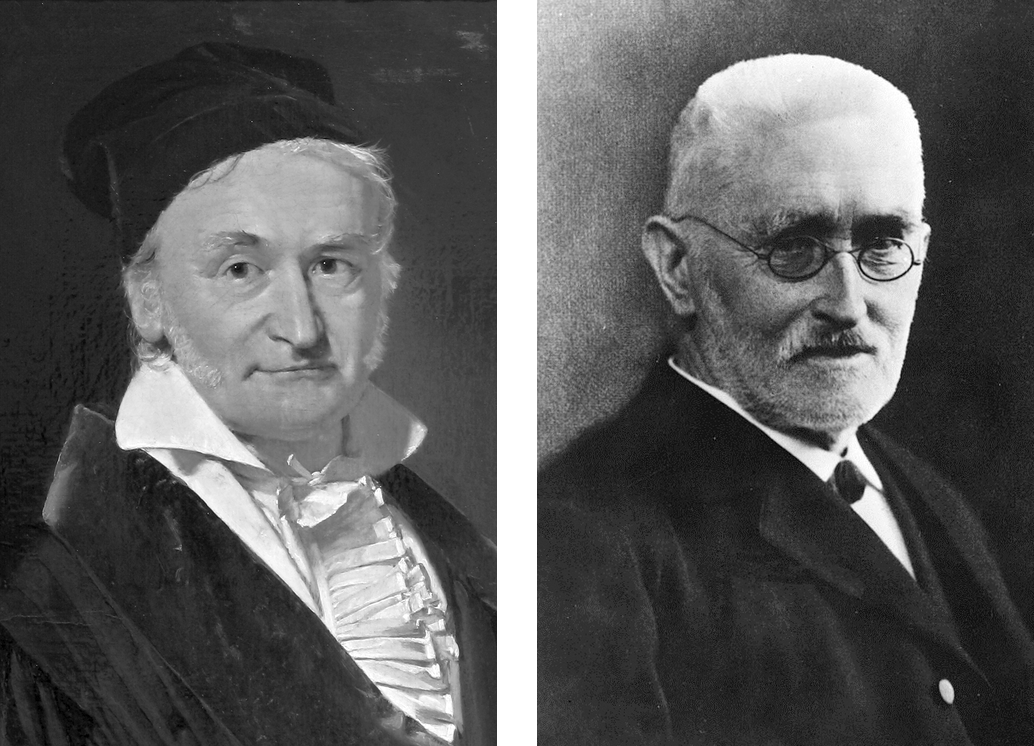
Carl Friedrich Gauss, left, and Richard Dedekind, right. Gauss selected Riemann’s difficult 1854 lecture topic on the foundations of geometry, while Dedekind later helped preserve Riemann’s legacy by publishing the lecture after Riemann’s death. Images via Wikimedia Commons: Gauss, Dedekind, public domain.

Riemann himself had hinted that geometry might ultimately belong to physics as much as to mathematics, but he did not live to see that possibility unfold.

For decades, his geometry waited inside mathematics.

Then Einstein needed it.

Charts, Atlases, And The Art Of Local Description

There is an everyday object that already teaches us how manifolds work. A map.

The Earth is curved, but a city map is flat. A map of Athens, Paris, or New York does not attempt to represent the entire planet perfectly. It describes one region. For that region, the flat approximation is useful.

But no single flat map can represent the whole Earth without distortion. Something must be sacrificed: distances, angles, areas, or shapes. This is why cartographers use different projections for different purposes.

Mathematicians use a similar idea for manifolds.

They cover a manifold with local coordinate systems called charts. Each chart describes one region using ordinary coordinates. Where two charts overlap, we need rules that tell us how to translate coordinates from one chart to another.

The collection of all these charts is called an atlas.

The word is perfect. Just as a geographical atlas contains maps of different regions of the Earth, a mathematical atlas contains coordinate descriptions of different regions of a manifold.

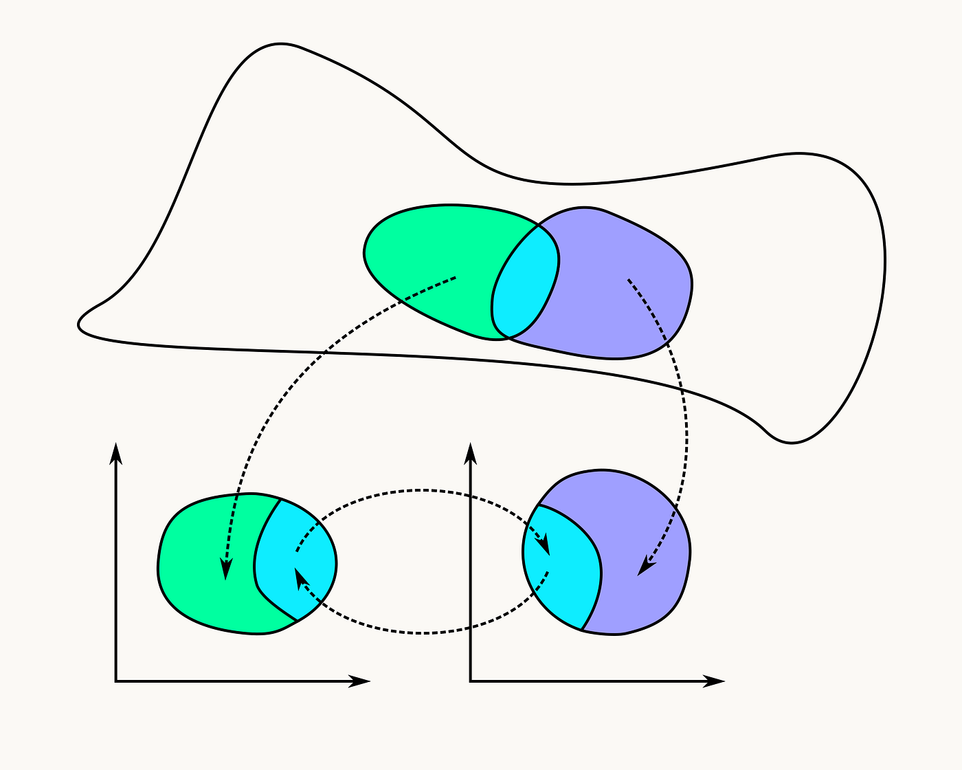
Two overlapping coordinate charts on a manifold. Each colored patch is represented by its own local coordinate system, and the dashed arrows indicate the transition maps that translate coordinates from one chart to the other. Image: Stomatapoll, Wikimedia Commons, licensed under CC BY-SA 3.0.

Atlases give us a way to navigate a manifold, but they do not yet give us geometry.

A small technical distinction hides here. A manifold gives us the local coordinate structure, the atlas of charts. To speak about distances, angles, shortest paths, and curvature, we need extra geometric structure, usually called a metric. A manifold equipped with such a metric is called a Riemannian manifold.

This distinction matters because coordinates alone do not give geometry. They tell us how to label points. A metric tells us how to measure.

With a metric, we can ask about lengths, shortest paths, angles, and curvature.

This is where manifolds become geometry.

Straight Lines On Curved Worlds

On a flat plane, the shortest path between two points is a straight line.

But what is a “straight line” on a sphere?

If you fly from one city to another, the shortest route usually follows part of a great circle, not a straight line drawn on a flat map. The equator is a great circle. Lines of longitude are also great circles. These curves are the sphere’s version of straight lines.

Mathematicians call such paths geodesics.

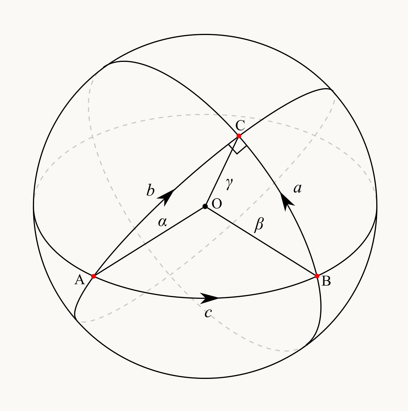
A spherical triangle drawn on the surface of a sphere. Its sides follow curved geodesic paths rather than straight lines in a flat plane. Image via Wikimedia Commons, public domain.

A geodesic is the natural generalization of a straight line to a curved space. It is a path that moves locally as straight as possible while remaining on the manifold. Locally, it is length-minimizing, although it may not always be the shortest route globally.

This last detail matters. A great circle route around the Earth is a geodesic in both directions. One direction may be the shorter route between two cities. The other may go the long way around the planet. Both still follow the same locally straight geometry.

On a plane, geodesics are ordinary straight lines. On a sphere, geodesics are great circles. On curved space-time, geodesics describe the paths of freely moving objects.

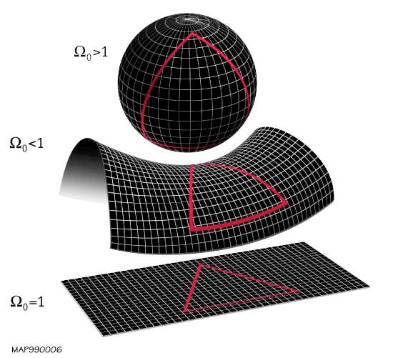
Geodesic triangles on surfaces with different curvature. Image: NASA/WMAP Science Team, Wikimedia Commons, public domain.

This is the bridge to Einstein.

Einstein did not arrive there in one clean step. For years, he struggled to find the right mathematical language for gravity. Around 1912, Marcel Grossmann helped point him toward the tensor calculus developed by Gregorio Ricci-Curbastro and Tullio Levi-Civita, the machinery needed to express curvature in a coordinate-independent way. The final field equations of general relativity emerged only after years of false starts, culminating in November 1915.

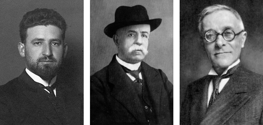
Marcel Grossmann, Gregorio Ricci-Curbastro, and Tullio Levi-Civita. Grossmann helped Einstein find the mathematical language of tensor calculus, built from the work of Ricci-Curbastro and Levi-Civita, that made general relativity possible. Images: Wikimedia Commons, public domain: 1, 2, 3.

In general relativity, gravity is not merely a force acting inside space. Mass and energy curve space-time, and freely moving bodies follow geodesics in that curved geometry.

In Newton’s picture, the Earth moves because the Sun exerts a force across space. In Einstein’s picture, the Sun changes the geometry of space-time, and the Earth follows a geodesic in that curved geometry. The orbit is no longer just motion through space. It is motion shaped by space.

As John Archibald Wheeler later put it, “Spacetime tells matter how to move; matter tells spacetime how to curve”.

The sentence is famous because it compresses a revolution.

Gravity became geometry.

Feeling Curvature Without Equations

Curvature can sound like a visual idea. A sphere looks curved. A flat sheet of paper does not. But in geometry, curvature is more than visual appearance. It is something that can be detected from within the space.

Here is one way to feel it.

Imagine drawing a small arrow on a flat sheet of paper. Move the arrow around a closed loop while keeping it as parallel to itself as possible. When it returns to the starting point, it points in the same direction as before.

Now imagine doing something similar on a curved surface, such as a sphere. Move an arrow around a closed loop while keeping it locally parallel along the way. When it comes back, it may not point in the same direction.

The arrow has rotated.

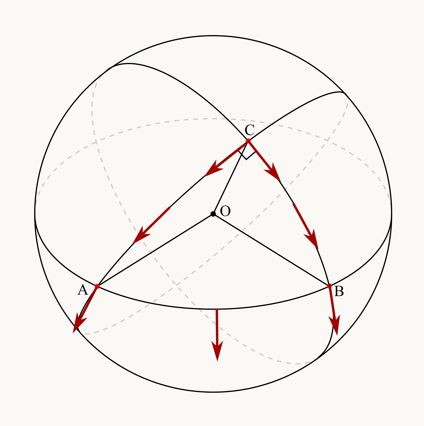
Parallel transport around a spherical triangle. The arrow is carried from C to A to B and back to C while kept locally parallel to the surface. When it returns to C, its direction has changed, revealing the curvature of the sphere. Adapted from a Wikimedia Commons diagram.

That rotation is not an accident. It is a sign of curvature. The size of the rotation measures how much curvature the loop encloses. For the spherical triangle above, the angle excess was 270 degrees minus 180 degrees, or 90 degrees; the transported arrow picks up the same 90-degree rotation.

On a flat surface, transporting an arrow around a loop brings it back unchanged. On a curved surface, the loop can reveal the geometry. Curvature is what makes the arrow remember the journey.

This gives a physical feeling to an otherwise abstract word. Curvature is not only what a surface looks like from the outside. It is something that can be measured by moving within the surface itself.

The universe does not need to be seen from the outside to have curvature.

Its curvature can be measured from within.

The Torus Hidden Inside A Double Pendulum

A manifold does not have to be a physical surface like the Earth. It can also represent a space of possibilities.

Consider a simple pendulum. To describe its position, we only need one angle. But angles repeat. An angle of 0 degrees and an angle of 360 degrees describe the same physical position. So the space of all possible angles is not a line. It is a circle.

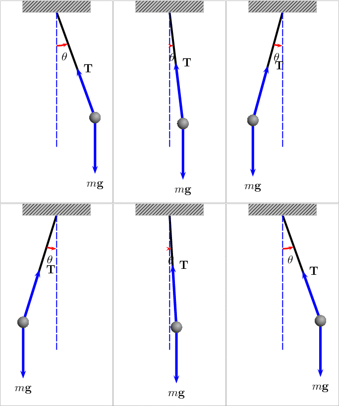
An oscillating pendulum with the angle θ measured from the vertical. The animation shows the tension T acting along the string and the weight mg acting downward on the mass. Image: Ruryk, Wikimedia Commons, licensed under CC BY-SA 3.0.

Now consider a double pendulum, where one pendulum hangs from the end of another. Its motion can look wild and chaotic. Small differences in the starting position may lead to very different paths.

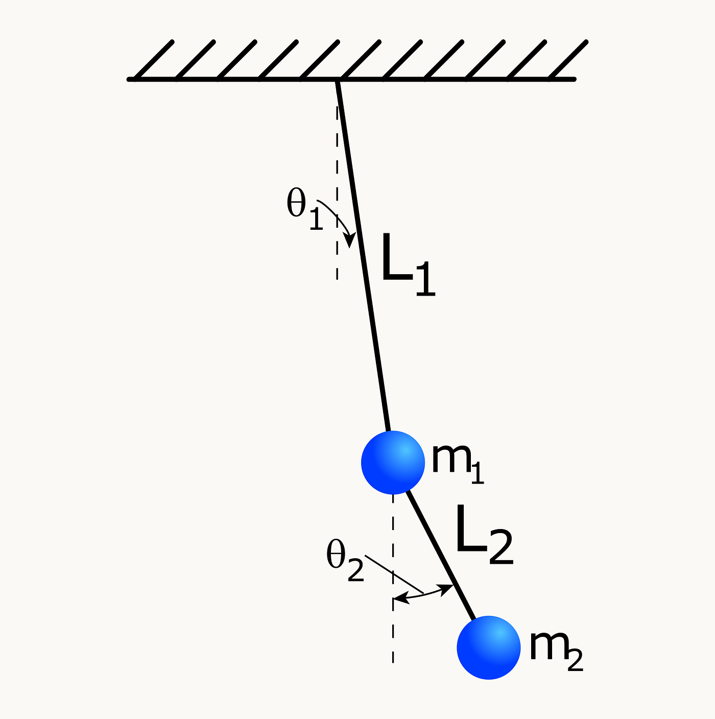
A double pendulum, made from two pendulums attached end to end. Image: JabberWok, Wikimedia Commons, licensed under CC BY-SA 3.0 and GFDL.

But at any instant, the configuration of the double pendulum can be described by two angles, θ₁ and θ₂. Each angle repeats after 2π, so θ₁ = 0 and θ₁ = 2π represent the same physical position, and the same is true for θ₂.

Now imagine drawing all possible pairs (θ₁, θ₂) inside a square. The horizontal direction represents θ₁. The vertical direction represents θ₂.

Because θ₁ repeats, the left and right edges of the square must be glued together. That gives a cylinder.

Because θ₂ also repeats, the top and bottom edges must also be glued together. That turns the cylinder into a torus, the surface of a doughnut.

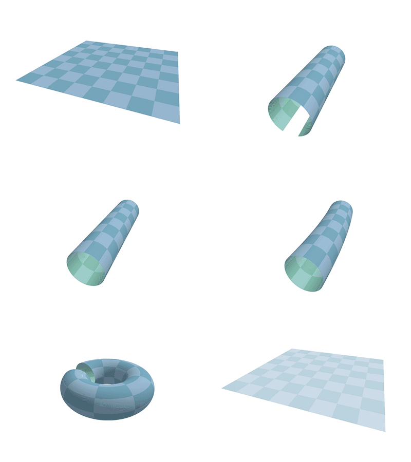
Animation showing how a square can be turned into a torus by first gluing one pair of opposite sides to make a cylinder and then gluing the remaining pair to form a doughnut shape. The checkerboard pattern makes the bending and distortion visible. Image: Lucas Vieira, Wikimedia Commons, public domain.

This is the hidden geometry of the double pendulum. The pendulum moves in physical space, but its configurations live on a torus. Each point on the torus represents one possible pair of angles. A motion of the pendulum becomes a path on this manifold.

The same idea appears in robotics. A robot arm with several rotating joints may move in three-dimensional space, but its possible configurations are described by joint angles. The set of all configurations forms a configuration space, often a manifold.

Planning the robot’s motion then becomes a geometric problem.

Which paths avoid obstacles? Which paths are efficient?

The Möbius Strip And The Surprise Of Global Shape

Some manifolds are locally ordinary but globally unsettling.

The Möbius strip is the classic example.

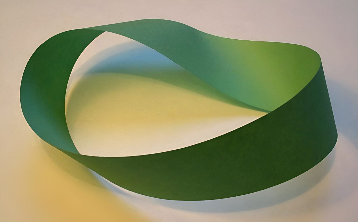
A paper Möbius strip made from a single band with a half-twist. Locally it looks like an ordinary strip, but globally it has only one side. Image: David Benbennick, Wikimedia Commons, retouched version uploaded by LukeTriton, licensed under CC BY-SA 2.0.

Make one by taking a strip of paper, giving it a half-twist, and taping the ends together. Near every point, the surface looks like a normal two-dimensional band. A tiny creature living on it would not notice anything strange locally.

But globally, the Möbius strip has only one side.

Start coloring one side of the strip and continue without lifting your pen. Eventually, you return to the starting point having colored what seemed to be both sides. The local picture never warned you that this would happen.

Local geometry does not always reveal global topology.

This is one reason manifolds became central to topology, the branch of mathematics that studies properties preserved under continuous deformation.

The Möbius strip reminds us that “flat nearby” does not mean “simple everywhere”.

Why High-Dimensional Data May Have A Hidden Shape

So far, the manifolds have been objects we can almost picture: spheres, strips, tori. But the same idea becomes even more powerful when the space is too large to visualize.

In modern, high-dimensional data, the manifold may be hidden inside thousands of coordinates.

A digital image may contain thousands or millions of pixel values. A sound recording may contain many time samples. A biological dataset may record the activity of thousands of genes or neurons. A language model may represent words or sentences using vectors with hundreds or thousands of components.

At first glance, such data seems to live in an enormous high-dimensional space.

But often, the data does not fill that whole space.

It lies near a lower-dimensional structure. That structure can often be thought of as a manifold.

Consider a grayscale image with 100 by 100 pixels. Each pixel has an intensity value between 0 and 1, from black to white. So the image is described by 10,000 numbers. Mathematically, each possible image is a point in a 10,000-dimensional space.

That sounds impossibly large.

But suppose the images are all pictures of the same handwritten digit, say the digit 3. Most points in that 10,000-dimensional space do not look like a 3. They look like random noise. The images that actually look like handwritten 3s occupy only a tiny, structured region.

The meaningful variation may be governed by a much smaller number of hidden parameters: thickness, slant, height, width, loop curvature, stroke pressure, rotation, and position. As those parameters vary smoothly, the corresponding images also change smoothly. The family of realistic handwritten 3s can therefore behave like a lower-dimensional manifold inside the much larger pixel space.

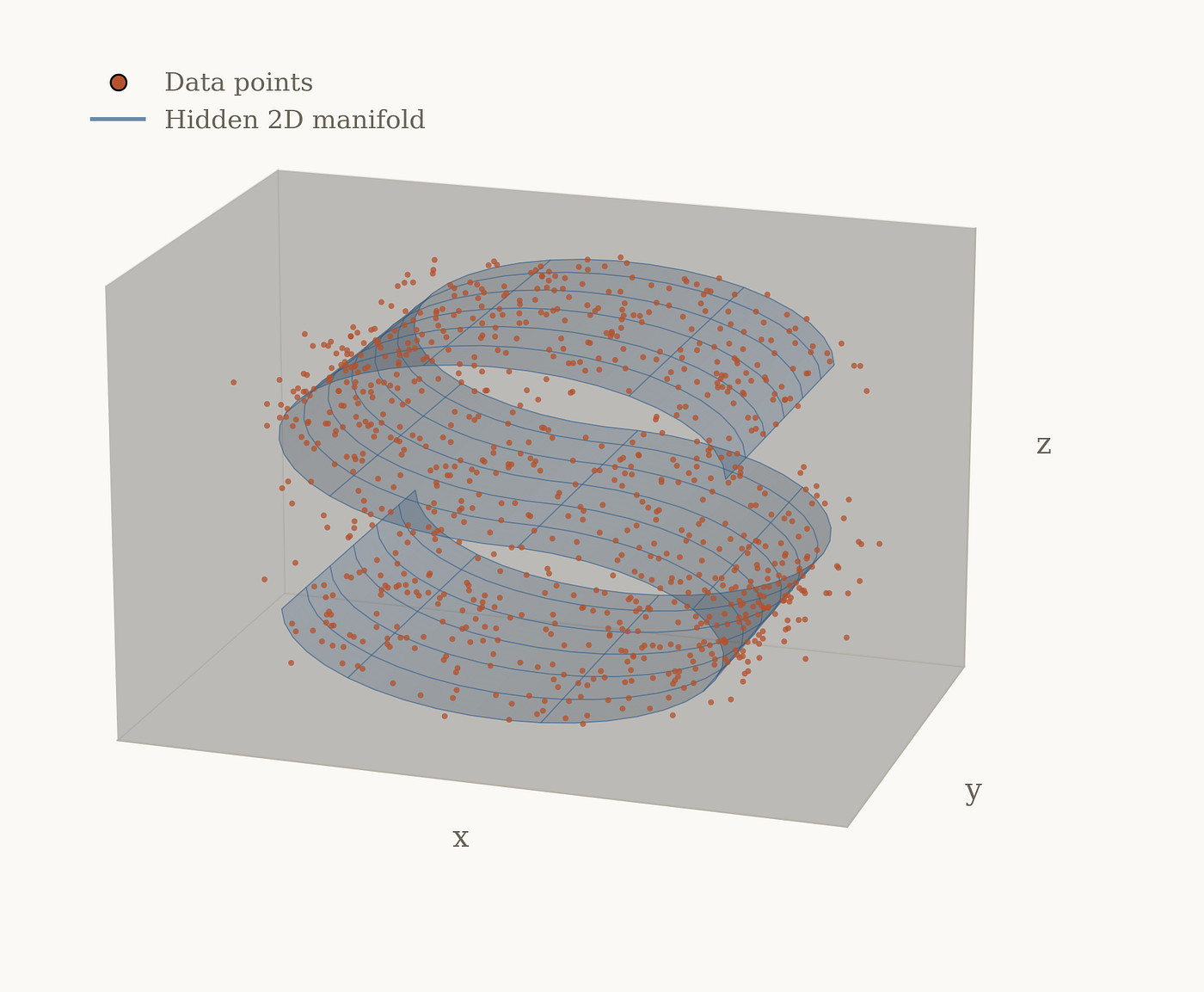
Data points may be stored in a high-dimensional space while lying near a much lower-dimensional hidden surface. The blue sheet represents a two-dimensional manifold, and the orange points represent noisy data clustered around it.

The Manifold Hypothesis

In machine learning, there is a common modelling assumption called the manifold hypothesis.

It says that many high-dimensional datasets are concentrated near lower-dimensional manifolds embedded in the high-dimensional space.

This is not a theorem that automatically applies to every dataset. It is an assumption, and like every modelling assumption, it can fail. But it is often useful.

The reason is simple. Real data is rarely arbitrary.

Images of faces are not random collections of pixels. Human speech is not random pressure variation. Sensor measurements from a physical system are not random points scattered everywhere. They are shaped by hidden causes, constraints, and degrees of freedom.

A face image may vary with pose, lighting, expression, age, camera angle, and distance. These variables are far fewer than the number of pixels in the image. A physical system may be measured by thousands of sensors, but its motion may be controlled by only a few dominant variables.

This is why dimensionality reduction can work. Principal component analysis (PCA) handles the case where the hidden structure is approximately flat. Methods such as Isomap try to preserve more of the manifold’s geometry. Algorithms such as t-SNE and UMAP are mainly visualization tools: they bend and compress high-dimensional relationships into two or three dimensions so that human eyes can see clusters and neighborhoods.

Finding hidden structure can help us classify images, detect anomalies, compress information, visualize complex datasets, or learn meaningful representations.

In this sense, machine learning is often not searching blindly through the full high-dimensional universe. It is trying to discover the hidden surface on which meaningful examples actually lie.

The Problem With Longitude At The Poles

One of the lessons of manifolds is that coordinates are not the same as the object itself.

A city can be described using latitude and longitude. It can also be described with a local street map, a postal address, or directions from a nearby landmark. These coordinate systems are useful, but they are not the city.

The same is true for manifolds.

A sphere can be described with latitude and longitude, but that coordinate system misbehaves at the poles. All longitudes meet there. This does not mean the sphere itself has a physical defect at the North Pole or South Pole.

The problem belongs to the coordinates, not to the surface.

This distinction matters in mathematics, physics, and data science, because it separates intrinsic structure from artifacts of description.

Sometimes the right question is not “What coordinates do we have?”

The better question is “What is the shape behind the coordinates?”

The Shape Behind The Coordinates

A manifold is the mathematical language of hidden order.

Complexity can emerge from simple local pieces, carefully stitched together.

Sometimes a space looks ordinary only because we are standing too close.