PCA: Proving the Magic with Pure Linear Algebra

We’ve all seen the advice. If you ask, “How do I become a great AI researcher?” the answer is always: “Master the foundations — Linear Algebra, Probability, Calculus, and Optimization.”

But what does “mastering” Linear Algebra actually mean? It’s a vague, daunting task. To make it tangible, let’s look at a real-world scenario. Imagine your boss hands you a dataset with 11 variables and says: “I need to visualize this in 2D, but there are no libraries allowed. Build it from scratch.”

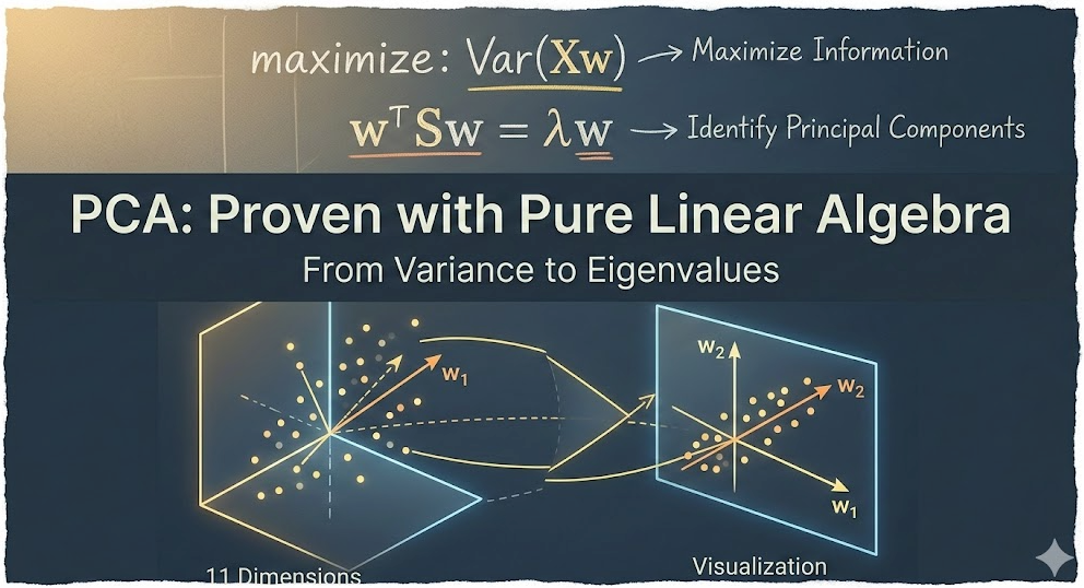
Your goal is to project high-dimensional data into a lower-dimensional space while capturing as much variance (information) as possible. This is exactly where Linear Algebra stops being a textbook chore and starts being a superpower. Without further due, let’s get into it.

Setting the Stage

Let our dataset X be represented as a matrix where rows are samples(n) and columns are features (d):

We want to project X onto a unit vector w. The goal is to maximize the variance of this projection. In math terms, we want to maximize:

The Setup: Centering the Data

To simplify the math, we assume X is mean-centered (the mean of each feature is 0). If X is centered, then its projection

is also centered.

Small challenge: Can you prove that if the mean of X is 0, then the mean of Xw is also 0? (Hint: Look at the sum of the elements in each column).

The Derivation

Since the mean is zero, the variance of our projection Xw is simply the average of the squared magnitudes:

Using the property of the L2 norm:

we can expand this:

By applying the transpose rule:

we get:

Notice the middle term?

is the Covariance Matrix(S). Now, our objective function is elegant and clean:

The Constraint

If we just try to maximize the previous equation without rules, we could just make w infinitely long to make the variance infinitely large. To prevent this “math breakdown,” we add a constraint where: w must be a unit vector.

Enter Lagrange

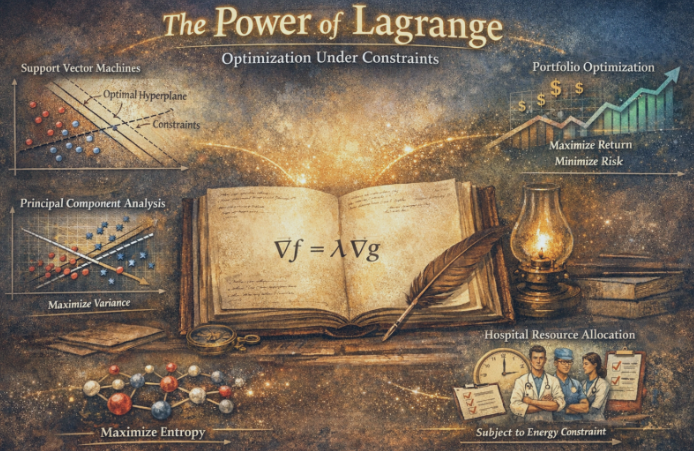
To solve a maximization problem with a constraint, we use the Lagrangian Multiplier, here’s a more detailed, deeper explanation of the intuition and insight behind Lagrange multipliers: https://medium.com/@giovanni.cortes75/the-hidden-treasure-in-a-valley-a-visual-guide-to-lagrange-multipliers-da950c871ea0.

To find the maximum, we take the derivative with respect to w and set it to zero:

Dividing by 2 and rearranging, we arrive at one of the most famous identity in Linear Algebra:

This is the ‘Eureka’ moment. We just proved that projecting high-dimensional data while preserving maximum information is simply a matter of finding the eigenvalues of S. No magic, no black boxes — just pure, undeniable Linear Algebra doing the heavy lifting for us, super beautiful. However, S can have several eigenvalues and eigenvectors, which one(s) to choose?

From One Vector to the Full Transformation

If our data has d dimensions, we have d potential vectors to choose from.

To project our 11-dimensional data, for example, down to 2 dimensions, we simply pick the two eigenvectors (w_1, w_2) associated with the two largest eigenvalues (λ_1, λ_2). These represent the directions of maximum “information” or variance.

The Matrix Global View

If we collect all our eigenvectors into a single orthogonal matrix W and our eigenvalues into a diagonal matrix λ, we can represent the entire system of equations at once.

Since S is a symmetric, positive semi-definite matrix, linear algebra guarantees that it can be diagonalized:

Where:

• W: A matrix whose columns are the eigenvectors (the principal components).
• Λ: A diagonal matrix where:

The eigenvalues or the amount of variance captured by each component

• WT: The transpose of W, which, because W is orthogonal, is also its inverse.

Let’s jump into a Google Colab notebook, build PCA from the ground up using nothing but NumPy, and put it head-to-head against Scikit-Learn!

Implementation

Let’s use an existing library for PCA

• Let’s use the famous iris dataset!

import numpy as np
import matplotlib.pyplot as plt
from sklearn.decomposition import PCA
from datasets import load_dataset

ds = load_dataset("scikit-learn/iris")
print('database info: ', ds)

database info:  DatasetDict({
    train: Dataset({
        features: ['Id', 'SepalLengthCm', 'SepalWidthCm', 'PetalLengthCm', 'PetalWidthCm', 'Species'],
        num_rows: 150
    })
})

• Let’s create a numerical category for the type of species.

df = ds["train"].to_pandas()
df['Species_Num'] = df['Species'].astype('category').cat.codes
df.head()

 Id SepalLengthCm SepalWidthCm PetalLengthCm PetalWidthCm Species Species_Num
0 1 5.1 3.5 1.4 0.2 Iris-setosa 0
1 2 4.9 3.0 1.4 0.2 Iris-setosa 0
2 3 4.7 3.2 1.3 0.2 Iris-setosa 0
3 4 4.6 3.1 1.5 0.2 Iris-setosa 0
4 5 5.0 3.6 1.4 0.2 Iris-setosa 0

• Let’s use sklearn PCA to capture as much variation as possible in the first component(highest eigenvalue and its respective eigenvector).

features = [
  'SepalLengthCm', 
  'SepalWidthCm', 
  'PetalLengthCm', 
  'PetalWidthCm'
]
pca = PCA(n_components=1)
X_pca = pca.fit_transform(df[features])
n = len(X_pca)

• Let’s visualize the first component and the type of the iris.

plt.scatter(range(0, n), X_pca, c=df['Species_Num'])
plt.ylabel("Principal Component 1")
plt.title("PCA Projection")
plt.show()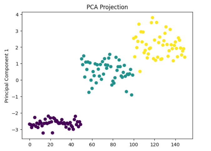

Let’s implement our own version of PCA

There only a few things we need to do based on our previous demostration:

• Mean-center our data.

df_mean_centered = df.copy()
df_mean_centered[features] = df_mean_centered[features] - df_mean_centered[features].mean()
df_mean_centered.head()

# Let's make sure the mean is cero
for feature in features:
    assert np.isclose(df_mean_centered[feature].mean(), 0), \
        f"Mean is not ~0 for {feature}"

• Calculate the covariance matrix(S) with the following formula.

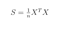
X = df_mean_centered[features].to_numpy()
cov_matrix = (1/n) * np.matmul(X.T, X)
cov_matrix

array([[ 0.68112222, -0.03900667,  1.26519111,  0.51345778],
       [-0.03900667,  0.18675067, -0.319568  , -0.11719467],
       [ 1.26519111, -0.319568  ,  3.09242489,  1.28774489],
       [ 0.51345778, -0.11719467,  1.28774489,  0.57853156]])

• Calculate the eigenvalues and eigenvectors for S, we will use a method from numpy.

eigenvalues, eigenvectors = np.linalg.eig(cov_matrix)
print('Eigen values: ', eigenvalues)
print('Eigenvectors values: ', eigenvectors)

Eigen values:  [4.19667516 0.24062861 0.07800042 0.02352514]
Eigenvectors values:  [[ 0.36158968 -0.65653988 -0.58099728  0.31725455]
 [-0.08226889 -0.72971237  0.59641809 -0.32409435]
 [ 0.85657211  0.1757674   0.07252408 -0.47971899]
 [ 0.35884393  0.07470647  0.54906091  0.75112056]]

• Project our data against the eigenvector with the highest eigenvalue.

# Let's use our model to calculate the projection of the data over the first

# Component, since looks like the np.linalg.eig is returning the values in order

# desc(may not always be the case but at least for this experiment we can take

# the first one)
X_custom_pca = np.matmul(X, eigenvectors[:, 0])

• Compare our graph with the sklearn solution.

plt.scatter(range(0, n), X_custom_pca, c=df['Species_Num'])
plt.ylabel("Principal Component 1")
plt.title("PCA Projection")
plt.show()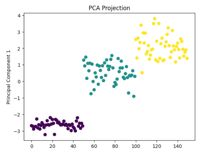

It’s one thing to see symbols on a page; it’s another to see them execute in code. As you can see from the plots, our manual implementation and Scikit-Learn’s PCA returned identical results.

Conclusion

Think about how powerful this is: we took a 4-dimensional dataset (the Iris flowers) and, using a single linear transformation, projected it onto a space where the different species are clearly separated and visible. Now, imagine the impact when you’re dealing with 11, 50, or more dimensions. Instead of drowning in a sea of variables, you’ve used Linear Algebra to distill the chaos into a clear, visual story. I hope you enjoyed this post!