Storage, Arbitrage, and the Structure of Energy Markets

Market Integration and Regime-Dependent Mean-Reversion in the US Energy Complex

An empirical cross-sectional study using FRED daily spot prices, 2000–2026

The Puzzle

Not all energy commodities absorb price shocks the same way. Some snap back to equilibrium quickly, others let a shock linger for months. This paper asks a specific question: within the US energy complex, does the speed of mean-reversion vary systematically with a commodity’s degree of global market integration and if so, is that relationship stable across macroeconomic regimes?

The answer, on FRED daily spot prices for nine US energy commodities which enter the cross-sectional analysis is yes. Globally referenced, storable products, crude grades and Gulf Coast distillates, mean-revert fastest. Regionally priced refined products sit in the middle. Pipeline-dependent Henry Hub natural gas is slowest. This ordering holds across both estimators tested, with Spearman rank correlations between integration and mean-reversion speed ranging from 0.855 (MLE) to 0.944 (AR(1)), both highly significant.

The relationship is not driven by any single macro environment. Estimating mean-reversion speed separately within each of four identified macro regimes, the integrated products show their highest mean-reversion speed in the post-2022 inflation-and-tightening regime, the strongest reading in the entire 25-year sample, while natural gas does not follow. But elevated mean-reversion also appears in the 2008–2013 crisis regime, when rates were near zero. This rules out a simple “higher rates, faster reversion” story and points instead to a subtler mechanism tied to the cost and feasibility of holding inventory under stress.

Background: Mean-Reversion and the Ornstein-Uhlenbeck Process

Unlike equities, most commodity prices exhibit mean-reversion, a tendency to return to a long-run equilibrium after a shock. This property is commonly captured by the Ornstein-Uhlenbeck (OU) process:

dX_t = kappa(mu - X_t)dt + sigma*dW_t

Where X_t is the log commodity price, mu is the long-run equilibrium, kappa is the mean-reversion speed, sigma is the diffusion coefficient, and W_t is a standard Brownian motion. The half-life of a price shock is ln(2)/kappa.

The OU specification should not be interpreted as a structural model of commodity prices over the full 25-year sample. We use it as a reduced-form approximation of local mean-reversion dynamics within identified macro regimes.

The central metric is the kappa-ratio: mean-reversion speed in the post-2022 regime divided by mean-reversion speed in the preceding New Normal regime (2013–2022). A ratio above 1.0 indicates faster mean-reversion in the recent regime, below 1.0, slower. The ratio measures how differently each commodity responded to the post-2022 regime relative to the low-rate decade that preceded it, it is a descriptive contrast between two regimes, not by itself a causal claim about what drove the change.

Two estimators, both reported. We estimate kappa using two methods: Maximum Likelihood (MLE) via the analytical OU solution, and AR(1) regression via OLS. Both are asymptotically equivalent under normality; differences arise primarily from MLE’s greater sensitivity to non-normal innovations including weather-driven price spikes. We treat neither as strictly correct, both are reported throughout as a robustness pair.

Data

Commodity spot prices: Daily spot prices sourced from FRED (Federal Reserve Bank of St. Louis), covering January 2000 to February 2026. Nine commodities across the US energy complex:

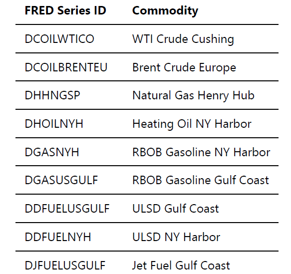
Why spot instead of futures. Continuous front-month futures series introduce roll gaps at contract transitions — artificial price discontinuities that bias OU estimation, particularly under MLE. Spot prices eliminate this contamination and permit direct interpretation of mean-reversion dynamics without roll mechanics.

Macroeconomic data: Daily US Treasury rates, monthly CPI, and monthly GDP from FRED, matching sample period.

Extreme-day treatment. Henry Hub natural gas exhibits three extreme single-day spikes over the sample corresponding to weather events: February 2021 (Winter Storm Uri), early 2024, and early 2025. These are physical delivery dislocations, not mean-reversion signals. Days with absolute log-returns exceeding 20% are winsorized before OU estimation. This affects fewer than 0.1% of observations and only for Henry Hub Natural Gas.

Methodology: Macro Regime Identification

Four macro regimes are identified via a two-stage unsupervised pipeline on monthly Treasury rates, CPI, and GDP. PCA reduces dimensionality; Gaussian HMM (warm-started from K-Means centroids via Hungarian algorithm) provides the final classification.

Stage 1 — Dimensionality reduction: PCA reduces the macro variable space to three components explaining approximately 85% of total variance.

Stage 2 — Regime classification: K-Means clustering provides an initial four-regime partition. A Gaussian Hidden Markov Model (HMM), warm-started from K-Means centroids via the Hungarian algorithm to avoid label-switching, refines the classification by imposing temporal persistence, consistent with the economic reality that macro regimes last months or years, not individual observations.

The two approaches agree on regime assignment in 93.8% of observations (Adjusted Rand Index: 0.845), with divergence concentrated at the three major macro transition points in the sample: 2008-2009, 2020, and 2022. This convergence across fundamentally different algorithms suggests the four-regime structure is a robust feature of the data. All subsequent OU calibrations use HMM regime assignments; K-Means results are reported as a robustness check.

Four regimes emerge without prior specification:

The clustering of 2020 with 2008-2013 is a notable validation: both periods share the same macro signature, zero rates, emergency liquidity, demand collapse despite different underlying causes.

FIGURE 1: Four macro regimes identified via Gaussian HMM on PCA components of US Treasury rates, CPI, andGDP. HMM warm-started from K-Means centroids via Hungarian algorithm. Agreement between methods:93.8% (ARI = 0.845). Divergence concentrated at 2008-2009, 2020, and 2022.

The Integration Score: Three Ex-Ante Binary Criteria

To avoid circularity, integration scores are constructed from three binary criteria defined ex ante, each grounded in externally verifiable sources. Each criterion is 0 or 1; the composite score ranges 0 to 3.

Criterion 1 — Global Benchmark Status. Does the commodity function as a globally referenced pricing benchmark in international trade contracts? Source: Fattouh (2011) An Anatomy of the Crude Oil Pricing System, OIES WPM 40, for crude classifications; IEA Oil Market Reports for refined products.

Criterion 2 — Global Specification Standardization. Does the commodity adhere to a globally harmonised technical specification, or does it exhibit regional variation?

Source: ASTM International Standards D975 (ULSD, equivalent to EN 590), D1655 (Jet Fuel, equivalent to DEF STAN 91–091), D4814 (Gasoline, US-regional with seasonal RVP variation), D396 (Heating Oil, primarily US).

Criterion 3 — Standard Storage Infrastructure. Can the commodity be stored in standard atmospheric-pressure tanks, or does it require specialised infrastructure?

Source: EIA Working Storage Capacity reports.

The four globally referenced commodities cluster tightly at 3.07–3.37. The regionally traded refined products (Heating Oil, RBOBs) cluster at 1.51–2.47. Henry Hub Natural Gas — the only fragmented market with pipeline-dependent regional pricing — shows the opposite direction, at 0.78.

Results

Kappa-Ratios Across the US Energy Complex

Kappa-ratios computed via AR(1) regression on winsorized daily spot prices, using HMM regime assignments:

The four globally referenced commodities cluster tightly at 3.07–3.37. The regionally traded refined products (Heating Oil, RBOBs) cluster at 1.51–2.47. Henry Hub Natural Gas — the only fragmented market with pipeline-dependent regional pricing — shows the opposite direction, at 0.78.

FIGURE 2: Commodities sorted by ratio, coloured by integration score

Absolute Kappa by Regime

The kappa-ratio contrasts two regimes, but the full picture requires the absolute mean-reversion speed in each of the four regimes. Estimating kappa separately within each regime shows where the cross-sectional ordering comes from and how it moves over time.

Two features stand out. First, in the post-2022 regime, the globally integrated products (WTI, Brent, Gulf Coast ULSD and Jet Fuel) reach their highest kappa of the entire sample, the visible peak on the right of the regime plot. Natural gas does not join them; its kappa is comparatively flat and sits below the integrated products in this regime. Second, elevated kappa for the integrated products also appears in the 2008–2013 crisis regime, despite near-zero rates in that period.

This second observation is the honest core of the result. If interest rates were the sole driver, the crisis regime should not show elevated mean-reversion. That it does points away from a pure rate-level mechanism and toward a common factor shared by both stress regimes: elevated cost or risk of holding inventory. In 2008–2013 that came through frozen credit lines and counterparty risk; post-2022 through financing costs. In both, holding inventory to sustain a price deviation became expensive, but only where physical arbitrage was possible at all.

FIGURE 3: Kappa by commodity across the four regimes

Cross-Sectional Statistical Evidence

Spearman rank correlations between integration score and kappa-ratio, computed under both estimators:

Both estimators produce highly significant positive correlations. The AR(1) estimator, more robust to non-normal innovations at the extremes of the price distribution, yields a stronger cross-sectional pattern. The MLE result, more sensitive to outliers but reported for methodological completeness, remains significant with a Jackknife minimum above 0.79.

The convergence of both estimators onto a positive significant Spearman across all diagnostic checks is the primary robustness result. Under neither estimator is the cross-sectional pattern eliminated by removing any single commodity.

FIGURE 4: integration score vs. kappa-ratio, with both estimators overlaid

Rolling Kappa Dynamics — and a Caution

Rolling OU kappa estimates using 756-day windows (three trading years) show how mean-reversion speed evolves continuously, as a complement to the discrete regime estimates.

Here the picture is more complicated, and it is worth being explicit about it rather than cherry-picking. The rolling estimates do not move in lockstep with interest rates. The most prominent rolling-kappa peaks for most commodities sit around 2008 and 2015 — the large oil price crashes — not at the 2022 rate peak. Overlaying the 1-month Treasury rate on the rolling kappas shows no clean co-movement.

Two things reconcile this with the regime results. First, a 756-day window blends data across regime boundaries: a reading dated 2015 contains 2013–2016 data, smearing the sharp regime transitions that the regime-level estimates preserve. The regime plot, which estimates kappa cleanly within each regime definition, is the appropriate basis for the cross-sectional claim; the rolling plot is context, not the primary evidence. Second, the rolling peaks coincide with the largest price dislocations in the sample, which is consistent with a reading that shock magnitude — not rate level — is a major driver of measured kappa in any given window.

What the rolling estimates do show robustly is the persistence of the cross-sectional ordering: across 2008, 2015, 2020, and 2022, the globally integrated products consistently exhibit higher mean-reversion amplitude than the fragmented markets. The relative ranking is stable even as the absolute levels move with each shock. That stability — not a co-movement with rates — is the temporal evidence for the structural interpretation.

Rolling kappa for Brent begins in September 2007, reflecting the 756-day estimation window and FRED daily data availability. No inference is drawn about the pre-GFC rate cycle from rolling estimates.

FIGURE 5: Integrated vs. fragmented commodities, overlaid with Treasury rates; note the absence of clean rate co-movement

Where r is the risk-free rate, u is storage cost, and y is convenience yield. The relevant quantity is the total cost of carrying inventory — financing plus physical storage — net of convenience yield. When carrying inventory becomes more expensive or riskier, the window over which arbitrageurs are willing to hold a position to close a price gap narrows, and deviations from equilibrium are corrected faster.

Crucially, carrying costs can rise for more than one reason. High interest rates raise the financing component directly. But a credit crisis raises the risk-adjusted cost of carry even at zero rates, frozen credit lines, counterparty risk, and collateral demands make holding inventory expensive in a different currency. This is why both the 2008–2013 crisis regime and the post-2022 tightening regime show elevated mean-reversion for the integrated products: both are high-carry-cost regimes, reached by different routes. The New Normal decade in between, cheap financing, functioning credit, low stress is precisely where mean-reversion is slowest.

This mechanism requires two conditions: physical storability and global price integration. Without storability, inventory cannot support arbitrage. Without global integration, arbitrage cannot close cross-regional price gaps.

Where the mechanism operates. WTI, Brent, and the Gulf Coast distillates (ULSD, Jet Fuel) satisfy both conditions. They are storable at scale in standard infrastructure and function as global pricing references. The carry-cost channel activates strongly in both stress regimes. Kappa-ratios cluster near 3.

Where the mechanism weakens. NY Harbor distillates and RBOB gasolines are storable but regionally priced due to US-specific specifications and refinery-hub logistics. Global arbitrage is partial. Kappa-ratios cluster near 1.5–2.5.

Where the mechanism fails. Henry Hub Natural Gas is neither globally integrated (pipeline-dependent, LNG-capacity-constrained) nor storable in standard infrastructure (underground caverns and aquifers only). The carry-cost channel cannot operate regardless of the rate or stress environment. Kappa-ratio: 0.78 — the opposite direction from the rest of the sample.

Alternative Explanations

Several alternative explanations are consistent with the observed pattern and cannot be excluded from price data alone.

Financing cost of speculative positions. Higher rates increase the cost of maintaining leveraged futures positions, reducing tolerance for holding loss-making positions and accelerating price convergence. This channel is not the same as the cost-of-carry mechanism but predicts the same directional effect. The two cannot be separated using price data alone.

Post-COVID supply chain normalisation. Global logistics capacity normalised in 2023–2024 after years of strain. For globally traded commodities, this may have reduced friction in physical arbitrage independently of interest rates.

Algorithmic trading intensity. Post-2022, algorithmic and systematic trading in commodity markets increased materially. This could accelerate mean-reversion through a microstructure channel rather than a cost-of-carry channel, particularly in the most liquid globally traded contracts.

Shock magnitude as a mechanical driver. Measured kappa is mechanically higher when large deviations from a stable mean revert quickly. The globally integrated products experience sharper, cleaner V-shaped shocks and recoveries; fragmented markets show noisier dynamics. Part of the cross-sectional ordering may therefore reflect the geometry of shocks in each market rather than an economic transmission channel. The rolling-kappa peaks around 2008 and 2015 — coinciding with the largest oil crashes — are consistent with this reading and should be taken seriously rather than explained away.

Transient overshooting. Regime 4 begins immediately after an extreme price shock. Elevated kappa could reflect transient reversion from overshooting rather than a structural shift. However, for Brent Crude — the strongest kappa-ratio commodity — elevated mean-reversion persists when the sample is restricted to mid-2023 onwards, after the acute 2022 shock had largely dissipated. This argues against a purely transient explanation for that commodity, though it does not rule out shock geometry contributing elsewhere.

Liquidity and market microstructure. Integration correlates almost perfectly with market depth and trading volume. Deeper markets may mean-revert faster simply because arbitrageurs can act sooner and in larger size. This channel predicts the same cross-sectional ordering and the same regime persistence, and cannot be separated from the carry-cost channel using price data alone. For a practitioner audience, it is arguably the more directly actionable interpretation.

Limitations

Sample size. n = 9 is statistically narrow. Ties within the score = 3 group (four commodities) reduce effective rank variation. Cross-commodity dependence within the energy complex further reduces effective degrees of freedom below n = 9.

Estimator sensitivity. Under different estimators, absolute kappa-ratios vary by 15–20%. The cross-sectional ranking is stable; magnitudes are not.

Data quality asymmetry. The three sources of data (Fattouh for benchmark status, ASTM for specifications, EIA for storage) are external and verifiable. The FRED price series varies in start date and reliability across commodities. Robustness to alternative data providers has not been tested.

Scope. All commodities are US energy products. The pattern does not extend to other commodity classes on this dataset. Generalising to metals, agriculturals, or non-US energy markets would require re-classification and separate estimation.

Rolling kappa convergence. For a substantial fraction of commodity-period combinations across the rolling analysis, OU convergence fails. This is itself informative — it identifies periods where OU is structurally inappropriate — but limits the temporal picture that can be drawn.

Causality. The cross-sectional pattern is consistent with cost-of-carry transmission but cannot establish causality on price data alone.

Implications for Practitioners

For energy derivative pricing: An OU model calibrated on pooled historical data is systematically miscalibrated in any regime that differs from the sample average — and the post-2022 regime differs sharply. Regime-conditional calibration differentiated by market structure corrects a systematic error whose direction can be anticipated from first principles.

For energy portfolio management: Cross-commodity hedges within the energy complex — particularly oil versus natural gas — assume a stability of relative dynamics that no longer holds post-2022. A portfolio treating oil and gas as substitutable energy exposures with similar mean-reversion behaviour is misspecified.

For refined product trading: The gap between globally referenced products (Gulf Coast ULSD, Jet Fuel) and regionally priced products (NY Harbor variants, RBOB) has widened in mean-reversion terms. Cracks and product spreads inherit this heterogeneity.

Conclusion

Within the US energy complex nine commodities entering the cross-sectional analysis we find a robust relationship between market integration and mean-reversion speed. Spearman correlations range from 0.855 to 0.944 across two estimators, with Jackknife minima above 0.79 in both. Every score assignment derives from an externally verifiable source: Fattouh (2011), ASTM International, and the EIA. The ordering is stable across macro regimes: integrated, storable products mean-revert fastest; fragmented Henry Hub natural gas slowest.

The regime-level estimates show that this ordering is most pronounced in stress regimes — both the 2008–2013 crisis and the post-2022 tightening — and weakest in the low-stress New Normal decade. This is consistent with a carry-cost mechanism in which the cost of holding inventory, whether raised by financing rates or by crisis-driven credit and counterparty risk, compresses arbitrage windows wherever physical arbitrage is possible. It is equally consistent with a liquidity-and-microstructure reading and with shock-geometry effects. The cross-sectional evidence does not distinguish cleanly between these channels; disaggregated position data or higher-frequency dynamics would be needed to do so. This paper deliberately does not claim that interest rates alone drove the pattern, the near-zero-rate crisis regime rules that out.

The practical implication is direct and does not depend on resolving the mechanism. Within the US energy complex, models that assume stationary mean-reversion parameters produce errors whose sign can be anticipated from the structure of each market and the prevailing regime. The choice between stationary and regime-conditional calibration is not a technical refinement, it is a substantive modelling decision with measurable consequences for pricing, hedging, and product-spread risk.

Data and Reproducibility

• Commodity spot prices (daily, 2000–2026): FRED via fredapi
• Macroeconomic data (Treasury rates, CPI, GDP): FRED
• Software: Python 3.11, hmmlearn, scikit-learn, statsmodels, scipy, arch
• Inflation adjustment: US CPI (FRED: CPIAUCSL)

References

1. Fattouh, B. (2011). An Anatomy of the Crude Oil Pricing System. OIES Paper WPM 40. Oxford Institute for Energy Studies.
2. Pirrong, C. (2012). Commodity Price Dynamics: A Structural Approach. Cambridge University Press.
3. Ng, V. K., & Pirrong, C. (1996). Price Dynamics in Refined Petroleum Spot and Futures Markets. Journal of Empirical Finance, 2(4), 359–388.
4. International Energy Agency (2024–2026). Oil Market Report. Monthly. Paris: IEA.
5. IMF Working Paper (2023). Monetary Policy Transmission through Commodity Prices.
6. Schwartz, E. (1997). The Stochastic Behavior of Commodity Prices: Implications for Valuation and Hedging. Journal of Finance, 52(3).
7. Hamilton, J. D. (1989). A New Approach to the Economic Analysis of Nonstationary Time Series and the Business Cycle. Econometrica, 57(2).
8. ASTM International. Standards D396, D975, D1655, D4814.
9. U.S. Energy Information Administration. Petroleum Supply Monthly and Working Storage Capacity Reports.

Benedict Hasenauer holds an MBA from Collège des Ingénieurs and the Certificate in Quantitative Finance (CQF).

All views expressed are the author’s own.