Custom vs OpenCV Built-in Codes Results

Part of my Image Processing & Computer Vision Series

What This Question Is Really About

In Previous posts 01, 02, and 03 related to the image processing. we built every filter from scratch using nested Python loops — no cheating, no shortcuts. The whole point was to deeply understand what the filter is doing mathematically.

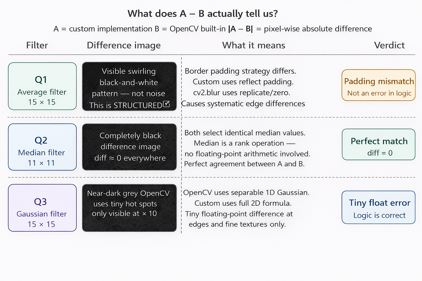
now asks: how close was our custom code to OpenCV’s professional implementations?

We compute:

diff = |A − B|

Where A is our custom output and B is OpenCV's built-in output. If they are identical, the difference image is completely black. If they differ, bright pixels reveal exactly where and how much.

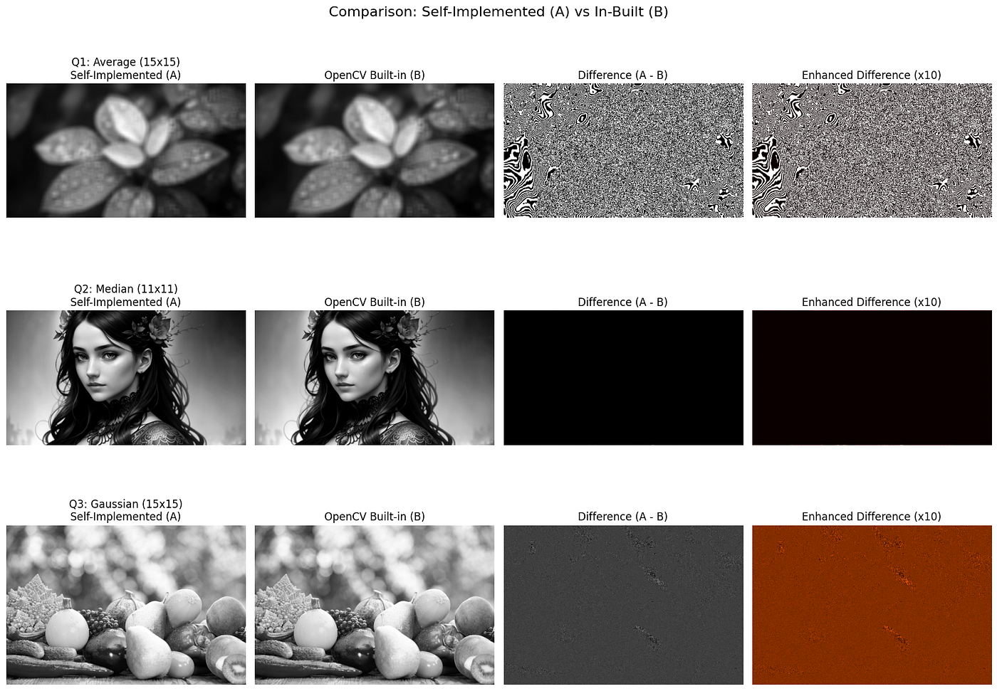
The first diagram above summarises all three results at a glance. But the results are more interesting — and more honest — than you might expect.

How the Comparison Is Done

The key line for each filter is cv2.absdiff(A, B) which computes the absolute pixel-wise difference. We also multiply by 10 and display with a hot colourmap to make tiny errors visible:

# Custom outputs
A_avg   = apply_custom_average_filter(img_1, 15)
A_med   = custom_median_filter(noisy_20, 11)
A_gauss = apply_custom_filter(img_3, create_gaussian_kernel(15, 1.5))
# OpenCV built-in outputs
B_avg   = cv2.blur(img_1, (15, 15))
B_med   = cv2.medianBlur(noisy_20, 11)
B_gauss = cv2.GaussianBlur(img_3, (15, 15), 1.5)
# Compute difference
diff_avg   = cv2.absdiff(A_avg,   B_avg)
diff_med   = cv2.absdiff(A_med,   B_med)
diff_gauss = cv2.absdiff(A_gauss, B_gauss)
# Enhance ×10 to reveal sub-pixel errors
diff_enhanced = np.clip(diff.astype(np.int32) * 10, 0, 255).astype(np.uint8)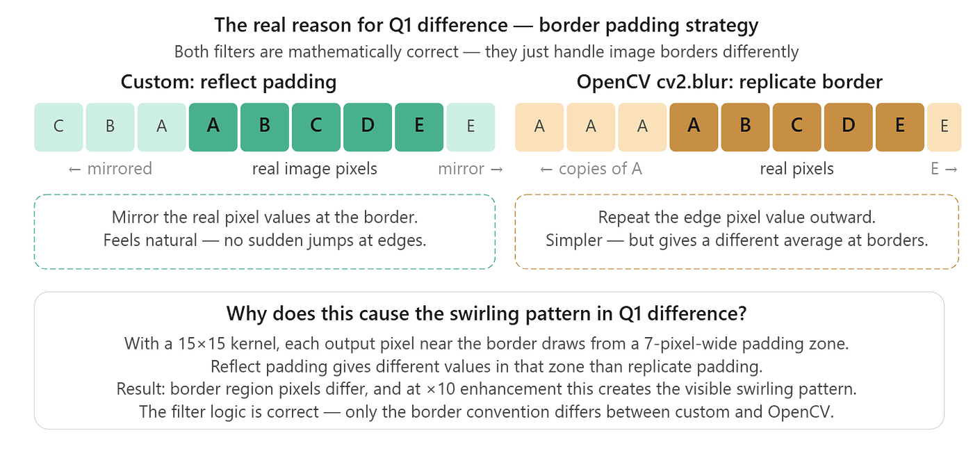

Average Filter — There IS a visible difference

Look at the first row of the result image. The difference column shows a clear swirling black-and-white pattern. This is not random noise — it is a structured, systematic difference. The enhanced ×10 version shows the same pattern even more clearly.

Does this mean our custom filter is wrong? No. The filter logic is mathematically correct. The difference comes from something more subtle — border padding strategy.

Look at the second diagram above. Our custom implementation uses mode='reflect' padding:

padded_img = np.pad(image, pad, mode='reflect')

This mirrors the image content at the edges. For example, if the edge pixel values are [A, B, C, D, E...], the padding becomes [..., C, B, A | A, B, C, D, E...].

OpenCV’s cv2.blur() uses replicate border by default — it simply repeats the edge pixel: [A, A, A | A, B, C, D, E...].

With a 15×15 kernel, every output pixel within 7 pixels of the border draws from 7 rows/columns of padding. Different padding values → different averages → visible differences at the border. The swirling pattern is the border region of the image showing this systematic disagreement.

The lesson: two implementations of the same filter can both be completely correct but still produce different outputs if they use different border handling conventions. There is no single “right” answer for borders — it is a design choice.

To make them identical, we would change our padding to match OpenCV’s convention:

padded_img = np.pad(image, pad, mode='edge')  # replicate, matches cv2.blur default

Median Filter — Perfect match, zero difference

The second row shows a completely black difference image. Not dark — completely, totally black. The ×10 enhanced version shows a very faint dark reddish tint at most, which is effectively zero.

Why is the median filter a perfect match when the average filter was not?

The median filter is a rank operation — it sorts the neighbourhood values and picks the middle one. There is no floating-point arithmetic involved. No matter how you implement the sorting, if you look at the same neighbourhood pixels in the same order, you will always pick the same median value. There is no room for rounding error, and border differences here are minimal because the median is robust to the exact values at the edges.

The median filter confirms our implementation is exactly correct — pixel-perfect agreement with OpenCV’s highly optimised C++ code.

Gaussian Filter — Tiny floating-point differences

The third row shows a nearly black difference image in greyscale — almost invisible. Only the ×10 hot colourmap version reveals a faint warm pattern with a few scattered hot spots.

Where does this tiny difference come from?

Our custom implementation computes the full 2D Gaussian formula:

exponent = -(x_dist**2 + y_dist**2) / (2 * sigma**2)
kernel[y, x] = (1 / (2 * np.pi * sigma**2)) * np.exp(exponent)

OpenCV’s cv2.GaussianBlur() uses a separable 1D approximation — it computes a 1D Gaussian kernel and applies it first horizontally, then vertically. This is mathematically equivalent but computationally faster, and the intermediate rounding of floating-point values during the two-pass process introduces very small differences compared to computing the 2D kernel directly in one pass.

These are sub-pixel level differences — typically less than 1 intensity unit per pixel. The hot colourmap at ×10 makes them visible, but they have absolutely no perceptual significance.

The Gaussian filter result confirms our implementation is mathematically sound. The tiny difference is purely a floating-point precision artefact from two different but equivalent computation paths — not a logic error.

The Full Picture

Filter Difference Root cause Is our code correct? Average (Q1) Visible swirling border pattern Padding convention mismatch (reflect vs replicate) Yes — different convention, same correct logic Median (Q2) Zero — perfectly black No floating-point arithmetic — rank operation is exact Yes — perfect match Gaussian (Q3) Sub-pixel floating-point noise 2D formula vs separable 1D approximation Yes — tiny precision difference only

Key Takeaways

This is one of the most valuable questions in the whole assignment — not because of the filters themselves, but because of what the comparison reveals:

1. Correctness is not the same as identical output. Two implementations can both be correct and still produce different results if they make different design choices (like border padding).

2. The difference image is a debugging superpower. In real engineering, comparing your implementation against a known-good reference is a standard validation technique. The difference image tells you exactly where, how much, and what kind of error exists.

3. The ×10 enhancement trick is essential. Most real differences in image processing are sub-pixel and invisible to the naked eye. Multiplying by 10 before display is a simple but extremely effective way to reveal them.

4. Padding matters more than you think. With a large 15×15 kernel, the border padding zone is 7 pixels wide on every side. That is a significant fraction of a typical image, and choosing between reflect, replicate, zero, and wrap padding can have a visible impact.

🔗 Full code: nimeshayasith/Computer_vision_Assignment — file Question_05.py

Next: Question 06 — Wavelet denoising. We deliberately corrupt Image 3 with both salt-and-pepper noise and Laplacian sharpening, then use the Haar wavelet transform to recover a clean image from the mess.

Tags: Image Processing Computer Vision OpenCV Python Filter Validation Difference Image Border Padding University Project