Advancements in Modern LLM Architectures

Latest LLM upgrades such as Mixture-of-Expert, RoPE, FlashAttention, Grouped-Query Attention, State Space Models (Mamba), Vision Language Models, RLHF and more.

In this short article, we will introduce you to the latest architectural and approach trends. In the following articles, we will follow each of these concepts in more depth. There are many new and experimental things, but the following are the ones that are actively used in the field in SOTA models.

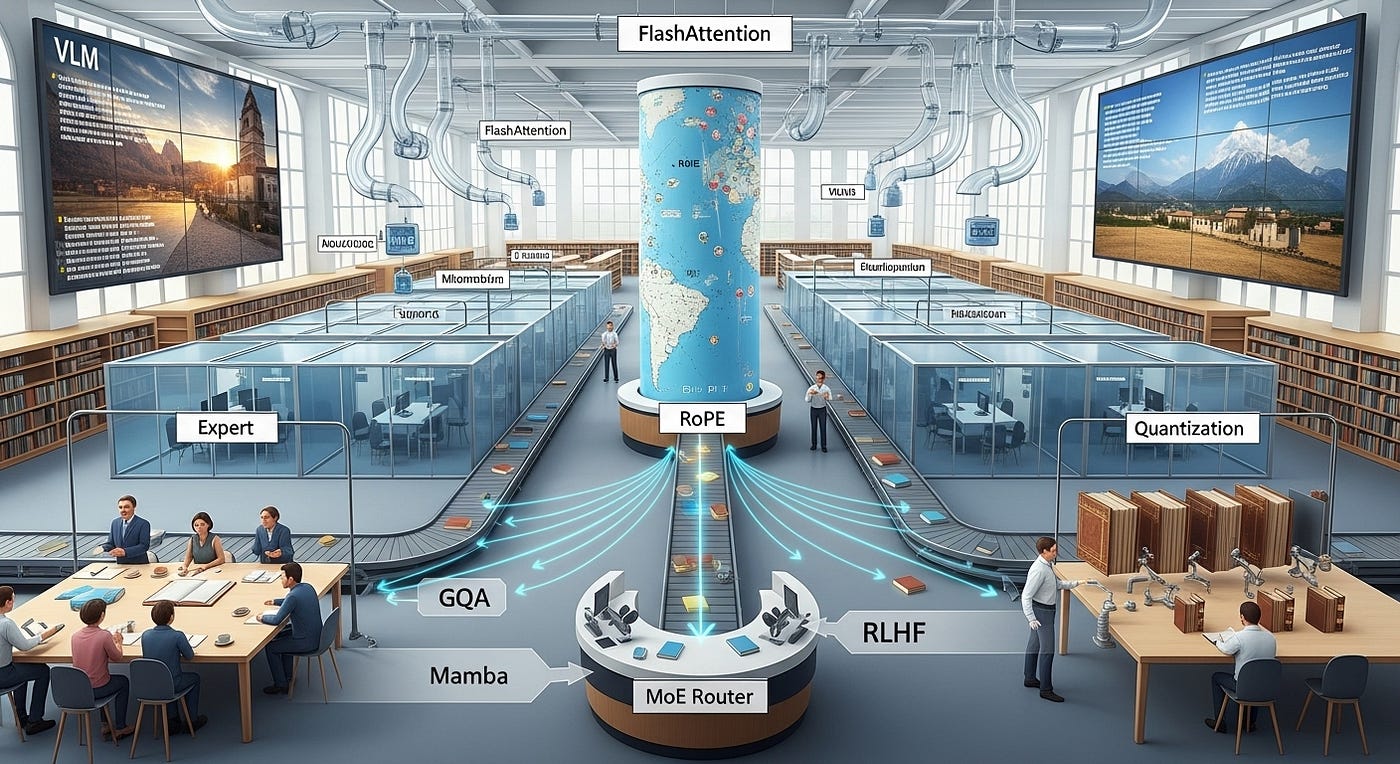
VLM is displayed on the screens; the cubicles represent expert nodes. The MoE router directs information to the appropriate expert cubicles. On the left, GQA is shown as a group of experts gathered around a table, while on the right, quantisation is showcased. The books symbolise information selected and refined by people through RLHF, the map represents RoPE, and Mamba serves as the conveyor belt.

Summary

This article provides a comprehensive overview of the key architectural innovations and optimisation techniques that have propelled the advancement of Large Language Models (LLMs) since the original Transformer. These advancements address critical bottlenecks in training cost, inference speed, context length, and model alignment, while also expanding capabilities into new modalities, such as vision.

• Mixture-of-Experts (MoE): Instead of a single large model, MoE uses a “router” to send input tokens to a selection of smaller, specialised “expert” networks. This allows models like Mixtral 8x7B to have a massive total parameter count (for knowledge) while only activating a fraction of them during inference, making it computationally efficient.
• Rotary Positional Encoding (RoPE): An elegant method for encoding word positions by “rotating” word embeddings in a vector space. Unlike older methods, it scales effectively to longer sequences and is utilised in models such as Llama and Gemma.
• FlashAttention: A low-level algorithm that dramatically speeds up and reduces the memory usage of the attention mechanism. It optimises data flow on GPUs by fusing operations and minimising slow memory I/O, enabling models to handle much longer contexts (e.g., 64k+ tokens) without approximation.
• Attention Variants (GQA): To solve the inference bottleneck of Multi-Head Attention (MHA), Grouped-Query Attention (GQA) offers a compromise. By having groups of query heads share a single key and value pair, it significantly reduces the memory footprint (KV cache) for faster inference with minimal loss in quality, becoming the standard in models like Llama 3.
• YARN (Yet another RoPE extension method): A technique to extend the context window of pre-trained models. It intelligently “stretches” RoPE’s positional encodings, allowing a model trained on a 4k context to operate effectively at 128k tokens with minimal additional training.
• State Space Models (Mamba): A new architecture challenging the Transformer. Mamba combines the linear-time inference speed of RNNs with the parallel training capabilities of Transformers. Its key innovation is a “selection mechanism” that allows it to contextually focus on important information, mimicking attention’s capabilities but with much better efficiency.
• Vision Language Models (VLMs): These models bridge the gap between text and images. They typically use a vision encoder (like ViT) to convert an image into “visual tokens,” a projector to align them with the text space, and an LLM to reason over both inputs. This enables powerful multimodal applications like visual question answering and image-based assistants.
• Quantisation: A suite of compression techniques (like GPTQ, AWQ, GGUF) that reduce the precision of a model’s weights (e.g., from 16-bit to 4-bit). This drastically shrinks the model’s memory footprint, making it possible to run massive LLMs on consumer hardware.
• Reinforcement Learning from Human Feedback (RLHF): The critical alignment step that teaches models to be helpful, harmless, and follow human preferences. The traditional method uses PPO, a complex process involving a separate reward model. A newer, simpler method called Direct Preference Optimisation (DPO) achieves similar results by directly training the model on a dataset of preferred vs. rejected responses, making alignment more stable and accessible.

Key Takeaways

1. Efficiency is the Driving Force: Many core advancements like MoE, GQA, and FlashAttention are not about creating a “smarter” algorithm but about making existing ones drastically more efficient. The goal is to scale models to trillions of parameters and handle massive context windows without prohibitive computational costs.
2. The Transformer is Being Challenged: While still dominant, the Transformer’s quadratic complexity is a major bottleneck. Mamba (State Space Models) represents the most promising alternative architecture, offering linear scaling and competitive performance, potentially defining the next generation of sequence models.
3. Inference Speed is as Important as Training: Techniques like GQA and Quantisation are primarily focused on inference. GQA reduces the KV cache bottleneck for faster token generation, while quantisation allows huge models to fit on smaller, more accessible hardware, democratising the use of powerful AI.
4. Context is No Longer a Hard Limit: The original ~2k token limit of early models has been shattered. Innovations like RoPE, FlashAttention, and extension methods like YARN are pushing context windows to hundreds of thousands of tokens, enabling LLMs to process entire books or codebases in a single pass.
5. Multimodality is the Future: The integration of vision and language through VLMs is a major step towards more general and capable AI. By learning to “see,” models can understand and reason about the world in a richer, more human-like way, unlocking countless new applications.
6. Alignment is Simpler and More Accessible: The shift from complex, multi-stage PPO to the more elegant Direct Preference Optimisation (DPO) has been transformative. DPO makes it significantly easier and more stable to align models with human values, allowing more teams to create safe and helpful AI without the massive engineering overhead of traditional RLHF.

If you are ready for more details, let’s begin.

The transformer architecture was invented in 2017, but the LLM era began more commonly; this is because a lot of new approaches were invented to decrease the cost of training and inference for these models and gain new modalities and capabilities. Let’s learn the ones that are the most influential.

1. Mixture-of-Expert (MoE)

Switch Transformers paper MoE layer

Instead of a single, monolithic “genius” model that handles every task, an MoE functions like a team of specialists. Imagine building a house: you hire a plumber, an electrician, and a painter, each an expert in their domain, rather than one person for all jobs.

1.1 MoE Architecture

An MoE model has two core components:

1. A Team of “Experts”: These are smaller, specialised neural networks (often replacing the Feed-Forward Network layers in a Transformer). Each expert becomes proficient at handling specific types of information.
2. A “Router” (or Gating Network): This is an intelligent manager that analyses incoming data (e.g., a token in a sentence) and decides which one or two experts are best suited to process it. For example, it might send the word “running” to an “action words” expert and “blue” to a “descriptive words” expert.

This design is highly efficient because for any given input, only a few experts are activated (“woken up”), saving immense computational power. It is also scalable, allowing for the creation of models with a vast number of total parameters (e.g., trillions) while keeping the computational cost of inference manageable.

1. 2. History and Evolution of MoEs

The concept dates back to a 1991 paper, “Adaptive Mixture of Local Experts,” based on a “divide and conquer” strategy. A key difference from simple ensemble models is the dynamic gating network that learns to route data intelligently.

MoEs regained popularity between 2010 and 2015 due to two key developments:

1. Conditional Computation: The idea that not all parts of a network need to be activated for every input. The path through the network can be dynamic and dependent on the data itself.
2. MoEs as Components: Instead of being the entire model, MoEs were integrated as layers within larger architectures, most notably replacing the Feed-Forward (FFN) layers in Transformers.

A landmark 2017 paper by Shazeer et al. scaled this concept to a 137 billion parameter model and introduced sparse top-k gating, a crucial innovation. Instead of calculating a weighted sum from all experts, the router selects only the top k experts (where k is a small number like 1 or 2). This “hard switching” enables sparsity and makes training massive models feasible.

However, scaling brought challenges like communication overhead in distributed training and load imbalance, where the router might favour a few “popular” experts, leaving others untrained. To solve this, an auxiliary load-balancing loss function was introduced to penalise the router for uneven token distribution.

1. 3. The Mechanics of Sparsity and Training

Sparsity in MoEs refers to sparse activation, not weight pruning. The core mechanism enabling this is the Noisy Top-k Gating algorithm:

1. Noise Injection: Trainable random noise is added to the router’s logits. This makes the routing stochastic and encourages exploration, preventing the router from always picking the same “favourite” experts.
2. Top-k Selection: Only the k experts with the highest scores are chosen. The scores for all other experts are set to negative infinity.
3. Final Softmax: A softmax function is applied to the modified scores, resulting in a sparse weight vector where only the top k experts have non-zero weights.

To manage the flow of data, the concept of Expert Capacity is introduced. This sets a limit on the number of tokens an expert can process in a single batch. If an expert is over capacity, tokens are “dropped” and passed to the next layer via a residual connection.

1.4 Fine-Tuning MoE Models

Fine-tuning MoEs presents unique challenges and insights:

• Overfitting: MoEs are more prone to overfitting than dense models. This can be mitigated with stronger regularisation, such as higher dropout rates within the expert layers.
• Knowledge vs. Reasoning: A key finding from the Switch Transformer paper is that when trained to the same level of general knowledge (perplexity), dense models perform better on reasoning-heavy tasks (e.g., SuperGLUE), while sparse MoEs excel at knowledge-intensive tasks (e.g., TriviaQA). The vast number of parameters in MoEs acts like a large, quickly accessible encyclopedia.
• Efficient Fine-Tuning: Surprisingly, freezing only the expert layers (which contain ~80% of the parameters) and fine-tuning the shared non-expert layers (like self-attention) yields results almost as good as fine-tuning the entire model. This is because updating the shared components has a more widespread effect on the model’s behaviour.
• The Power of Instruction Tuning: A recent paper, “MoEs Meet Instruction Tuning,” found that MoEs benefit far more from instruction tuning (fine-tuning on a wide mix of diverse tasks) than dense models do. This diverse training appears to be the perfect catalyst to leverage the specialised expert architecture. The study also found that keeping the auxiliary load balancing loss active during this process is crucial to prevent overfitting.

1.5 Practical Considerations and Future Directions

• Use Cases: MoEs are ideal for high-throughput scenarios with ample hardware. For low-throughput or VRAM-constrained environments, a dense model is often more practical.
• Parallelism: “Expert Parallelism” is a common strategy where different experts are placed on different devices (GPUs/TPUs), and tokens are routed across the network to their assigned expert.
• Inference Techniques: To make large MoEs practical for deployment, techniques include:
• Distillation: Training a smaller, dense model to mimic the behaviour of a large MoE.
• Expert Aggregation/Merging: Combining the weights of multiple experts to reduce the total parameter count during inference.
• Efficient Training Frameworks: Projects like FasterMoE and Megablocks have developed optimised GPU kernels and communication strategies to speed up MoE training significantly.
• Open-Source Models: Several powerful MoE models are now open-source, including Google’s Switch Transformers, Meta’s NLLB MoE, and Mistral’s Mixtral 8x7B, which outperforms Llama 2 70B with much faster inference.
• Future Research: Exciting areas include further experiments in distillation, model merging, and quantisation. The QMoE paper demonstrated extreme quantisation, compressing a 1.6 trillion parameter model from 3.2 TB down to just 160 GB.

For more details, please check (it is Turkish, but you can translate the page or check out its sources):

[embed]MoE: Uzman Karması (Mixture-of-Experts) MoE’lerin yapısını, nasıl eğitildiklerini ve çıkarım amacıyla kullanılırken dikkate alınması gereken ödünleşimleri…medium.com

2. RoPE (Rotary Positional Encoding)

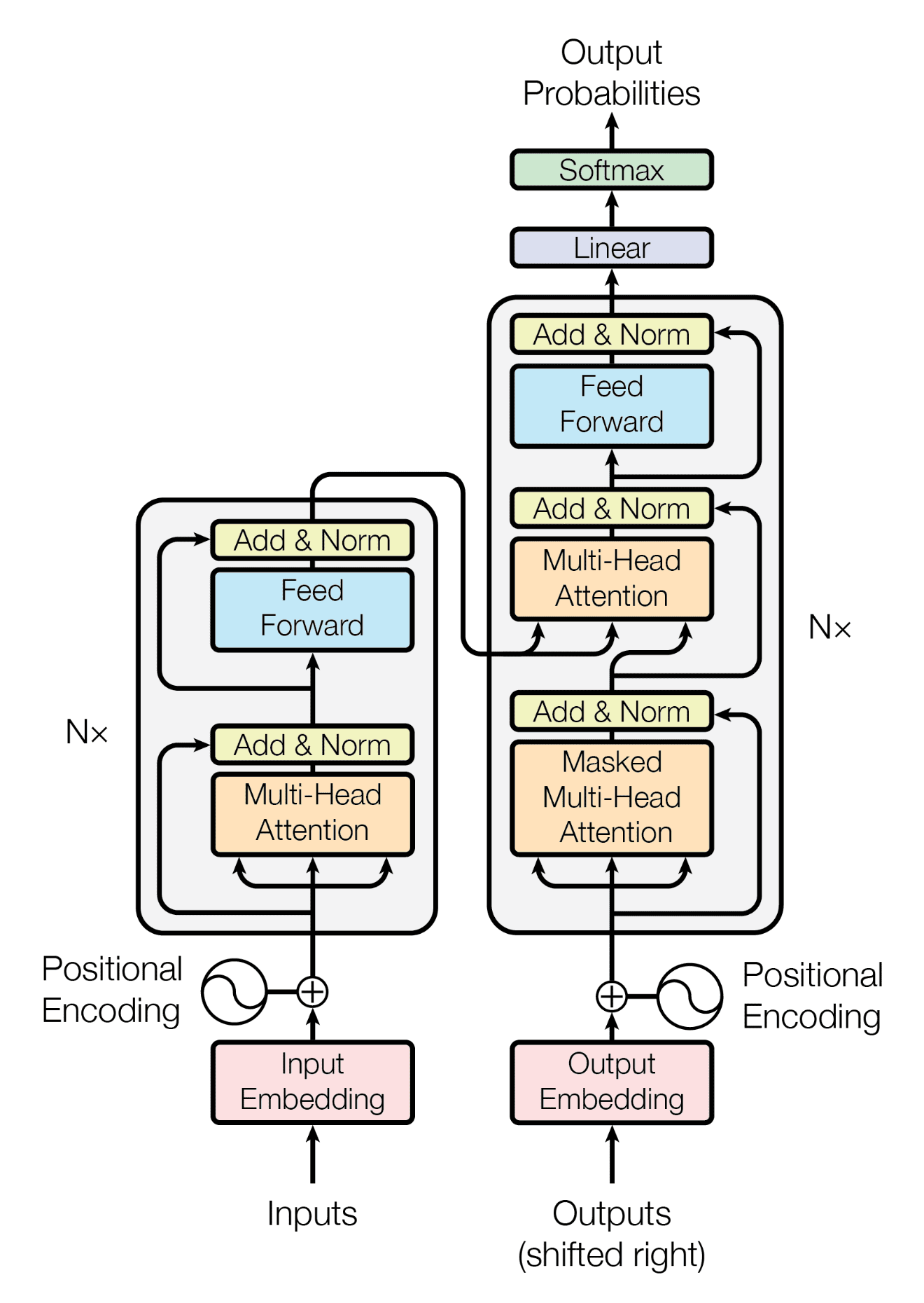
The + parts after embeddings is the positional encoding layer.

Words placed in a sentence change the meaning, so we need to encode the positions of the words. The “Attention is All You Need” paper in 2017 contains a positional encoding layer, and in that layer, sinusoidal positional encodings are used, which are fixed, deterministic functions of position that are added to the input embeddings before being fed into the self-attention layers.

In 2021, the “RoFormer: Enhanced Transformer with Rotary Position Embedding” [https://arxiv.org/abs/2104.09864] paper introduced RoPe, an approach that applies rotations directly in the query and key vector spaces during attention computation, rather than adding position vectors to token embeddings. RoPe is currently used by the Llama and Gemma models.

Types of Positional Embeddings

1. Absolute Positional Embedding

Imagine giving every word a unique sticker based on where it appears in a sentence. That’s absolute positional embedding — it assigns a fixed position to each word. It works great for sequences of the same length, but struggles when dealing with longer sequences than seen during training.

2. Relative Positional Embedding

Instead of assigning a fixed position, this method focuses on how far apart words are. Think of it like a game of ‘who’s closer’ rather than ‘who’s first’! It is more flexible and works well with different sequence lengths. But it adds extra computation because it modifies the attention scores.

3. Rotary Positional Embedding

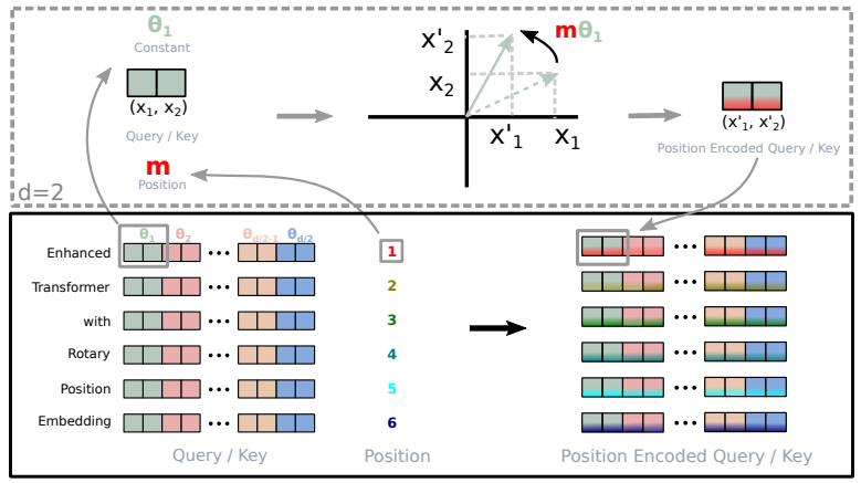
The implementation of the RoPE

RoPE is like giving each word a spin in a multi-dimensional space! Instead of learning positional values or adjusting attention scores, RoPE rotates word embeddings in a way that naturally encodes their position.

RoPe can:

• Handle longer sequences well. No more worrying about unseen lengths!
• Computationally efficient. No extra parameters, no tweaking attention scores!
• Improves long-range understanding because context matters!

3. FlashAttention

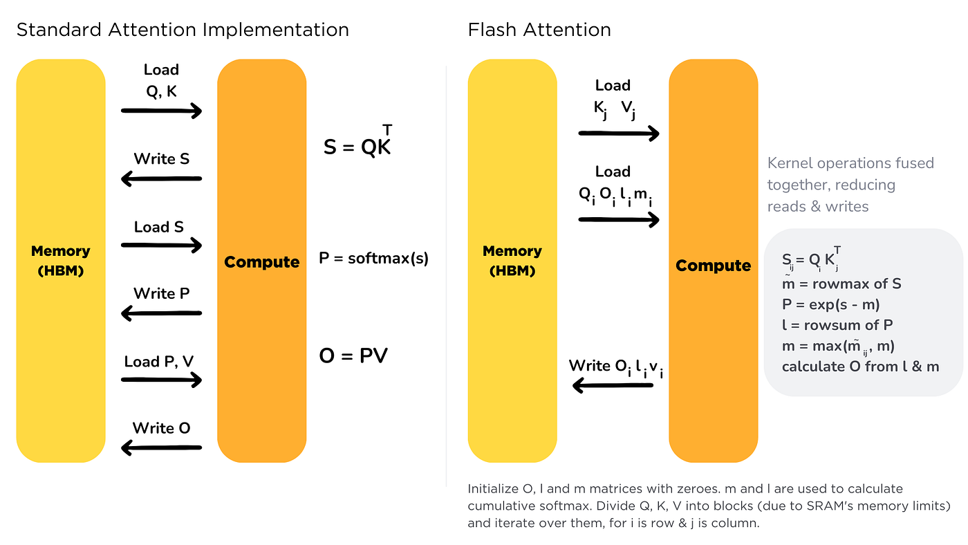
FlashAttention is an optimised algorithm designed to significantly accelerate and improve the memory efficiency of the self-attention mechanism in Transformers. Scaling Transformer architectures is heavily bottlenecked by self-attention, which has quadratic time and memory complexity with respect to sequence length. While modern accelerators (like GPUs) have improved in compute capacity, their memory bandwidth and data transfer speeds have not scaled at the same rate. This leads to a memory bottleneck in attention operations.

FlashAttention addresses this issue by rethinking how attention is computed and how data is moved between different levels of GPU memory.

3.1 Standard Attention and the Memory Bottleneck

In the standard attention implementation, the keys (K), queries (Q), and values (V) are stored, read, and written repeatedly from High Bandwidth Memory (HBM) — the large but relatively slow memory on a GPU. The process typically involves:

1. Loading Q, K, V from HBM into the on-chip Static RAM (SRAM) (which is much faster but smaller).
2. Performing a partial attention computation.
3. Writing intermediate results back to HBM.
4. Repeat this process for every step in the attention operation.

This repeated loading and storing creates a large memory transfer overhead, dominating the runtime despite GPUs having ample compute capability.

3.2 How FlashAttention Works

FlashAttention optimises this process by:

• Tiling and streaming: Dividing the attention computation into smaller blocks (tiles) that fit entirely within GPU SRAM.
• Fusing operations: Instead of writing intermediate results to HBM after each sub-step, FlashAttention performs all steps of the attention mechanism (matrix multiplication, scaling, softmax, dropout, etc.) within a single fused kernel while data remains in fast SRAM.
• Minimising memory I/O: Q, K, and V are loaded once from HBM, processed completely in SRAM, and then written back only once at the end.
• Maintaining exactness: Unlike approximate attention methods, FlashAttention computes the same output as standard attention by carefully maintaining numerical stability using log-sum-exp accumulation.

This dramatically reduces data movement between HBM and SRAM, which is the true bottleneck in attention computation.

3.3 Advantages and Disadvantages

Advantages

1. Speed: Up to 2–4× faster training and inference for long sequences.
2. Memory Efficiency: Uses up to 10–20× less memory by avoiding the explicit creation of the full attention matrix QKTQK^TQKT.
3. Exact Output: Produces mathematically identical results to standard attention.
4. Better GPU Utilisation: Keeps most data within high-speed SRAM, avoiding slow HBM read/writes.
5. Scalability: Enables training and inference with much longer sequence lengths (8K–64K tokens or more).

Disadvantages and Limitations

1. Implementation Complexity: Requires custom CUDA kernels; significantly harder to modify or extend.
2. Hardware Dependency: Optimised for NVIDIA GPU architectures; less portable to CPUs or non-NVIDIA accelerators.
3. Limited Flexibility: Early versions do not support all attention variants (e.g., certain sparse or cross-attention types).
4. Precision Sensitivity: Although numerically stable, small differences can appear in extreme cases or mixed-precision training.
5. Dependency on Frameworks: Requires compatible frameworks such as PyTorch 2.0+ or the flash-attn library.

Evolution

1. FlashAttention v1 (2022): Introduced tiled, exact attention with fused kernels.
2. FlashAttention v2 (2023): Faster kernels, supports more attention types (causal, multi-query).
3. FlashAttention v3 (2024): Optimised for NVIDIA Hopper GPUs, supports variable-length batching and rotary embeddings.

4. Multi-Head Latent Attention (MLA), Group Query Attention (GQA), Multi-Query Attention (MQA) and Multi-Head Attention (MHA)

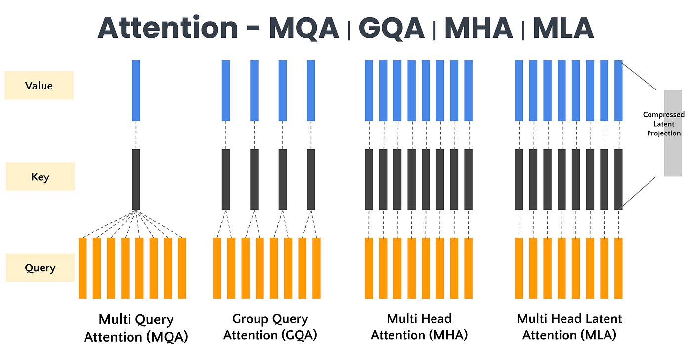
Here is a summarised comparison as a table:

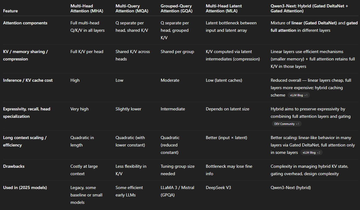
In 2025, Grouped-Query Attention (GQA) has become the default choice for most large open-weight models like LLaMA 3 and Mistral, offering an optimal balance between efficiency and expressivity by sharing keys and values across head groups to reduce memory use without much accuracy loss. Multi-Query Attention (MQA) remains favoured for ultra-fast inference in production APIs but is less expressive, while Multi-Head Latent Attention (MLA), used in DeepSeek V3, pushes efficiency further by compressing key–value states through latent representations — ideal for very long contexts and large-scale serving. Meanwhile, Qwen3-Next pioneers a new hybrid gated attention that mixes linear (DeltaNet) and standard attention layers, achieving even higher throughput for long-context tasks. Overall, GQA is preferred for balanced general-purpose models, MLA for ultra-efficient long-context or multimodal systems, and Qwen-style hybrid attention for cutting-edge MoE architectures emphasising both speed and stability.

Analogies to Ease Remembering

Once upon a time, there was a team of detectives 🕵️‍♂️ trying to solve a huge mystery (the task of modelling relationships between all tokens in a sequence).

• Multi-Head Attention (MHA): Each detective had their own magnifying glass 🔍 (their own query projection Q) and checked every single clue 📄 (all keys K and values V) on their own. This meant every clue was examined from a unique perspective (maximum expressivity), but it took a long time, and the office was cluttered with notes (high memory and compute cost).
• Multi-Query Attention (MQA): Then, they tried a new approach. Each detective still looked in a different direction (different queries Q), but they all shared the same master notebook 📖 (shared K/V across all heads). This was much faster and lighter (less memory/computation), but sometimes small details were missed (slight loss of representational diversity because all heads see the same K/V).
• Grouped-Query Attention (GQA): To balance speed and thoroughness, detectives formed small teams 👥, each with their own notebook (groups of heads sharing K/V). Now, each group could specialise while still saving memory, so more clues were caught without everyone duplicating effort (good trade-off between efficiency and expressivity).
• Multi-Head Latent Attention (MLA): Later, they hired a clever intern 🧑‍💻 who made a summary cheat sheet 🗂️ of all the clues (latent vectors compressing the full input K/V). Detectives could consult the cheat sheet instead of re-reading every clue. Super fast for huge mysteries (efficient scaling for long sequences), but tiny hints might be lost (some fine-grained information is compressed).
• Qwen3-Next Hybrid Attention: Finally, they adopted a hybrid car 🚗 approach. Most of the time, the team used the intern’s cheat sheet (linear Gated DeltaNet layers for efficiency) to move quickly across easy terrain, but whenever they hit a tricky puzzle, they switched to full detective mode (gated standard attention layers) to make sure no clues were missed. This gave them both speed and precision (high throughput for long contexts while maintaining expressivity).

The original Transformer paper introduced Multi-Head Attention (MHA), a mechanism that allows the model to attend to information from multiple representation subspaces in parallel. In contrast, Multi-Head Latent Attention is a more recent architectural innovation designed to overcome the quadratic computational and memory complexity of standard self-attention. It enables transformers to efficiently process extremely long sequences such as high-resolution images, long documents, audio, or video streams by introducing a small, fixed set of latent vectors that act as an intermediary bottleneck. Rather than computing attention between every pair of input tokens, the model attends from the inputs to these latent vectors (and vice versa), effectively summarising and refining the information. This latent attention mechanism forms the core of architectures like Perceiver and Perceiver IO.

4.1 The Problem with Standard Attention in Large Contexts

Standard self-attention has a time and memory complexity of O(n²), where n is the sequence length. This makes it computationally infeasible for inputs with tens of thousands or millions of tokens. For example, a single 224x224 image already contains over 50,000 pixels (tokens). Applying standard self-attention directly would be prohibitively expensive. This bottleneck fundamentally limits the ability of standard transformers to handle high-bandwidth, multi-modal data.

4.2 How Multi-Head Latent Attention Works

This architecture decouples the main model depth from the input sequence length by introducing a small latent array. The process generally involves two key steps using cross-attention:

1. Input Compression (Encoding): A cross-attention mechanism is used to compress the massive input sequence into a small, fixed-size latent array.

• Queries (Q): The latent vectors act as the queries.
• Keys (K) and Values (V): The input token embeddings provide the keys and values. This step effectively “asks” the input sequence for its most important information and distils it into the latent array.

2. Processing in Latent Space: The model then applies a deep stack of standard (and computationally cheap) self-attention layers only on the small latent array. This allows the model to process and reason about the summarised information from the input without ever paying the O(n²) cost of the full sequence.

3. Output Generation (Decoding): To produce an output, another cross-attention layer is used. A task-specific query vector queries the processed latent array to extract the necessary information and generate the final result.

The “Multi-Head” aspect simply means that each of these attention steps (cross-attention and self-attention) uses multiple heads to capture different features and relationships, just like in a standard transformer.

4.3 Advantages and Disadvantages

Advantages

• Scalability to Massive Inputs: Breaks the O(n²) bottleneck, allowing transformers to process inputs of virtually any size, as complexity scales with the input size n and latent array size m (O(nm)), where m is much smaller than n.
• Modality Agnostic: Can handle diverse data types (images, text, audio, point clouds) by first projecting them into a common representation. The latent array then processes this representation, making the architecture highly flexible.
• Computational Efficiency: The bulk of the computation occurs in the small latent space, making the model very deep and powerful without being prohibitively expensive.
• Parameter Efficiency: The core processing block is independent of the input size, allowing for more efficient parameter usage.

Disadvantages and Limitations

• Information Bottleneck: By its nature, compressing a large input into a small latent array is a lossy process. Fine-grained details from the original input may be lost, which can impact performance on tasks requiring high fidelity.
• Architectural Complexity: The design, involving multiple stages of cross-attention and self-attention, is more complex to implement and reason about than a standard encoder-decoder transformer.
• Niche Application: It is a fundamental architectural choice, not a drop-in optimisation like GQA or FlashAttention. It is primarily used in specialised models designed for multi-modal or very-long-sequence tasks.
• Potential for Blurring Details: The abstraction might cause the model to “blur” distinct but similar features, as it is forced to create a generalised summary in the latent space.

4.4 Grouped-Query Attention

Grouped Query Attention (GQA) is an optimisation of the standard multi-head attention mechanism designed to offer a balance between the high performance of Multi-Head Attention (MHA) and the inference speed of Multi-Query Attention (MQA). It was developed to reduce the significant memory bandwidth overhead of large language models during inference, making them faster and more efficient without a major sacrifice in accuracy.

GQA has been widely adopted by Meta Llama 3, Mistral 7b and 8x7b and IBM Granite series LLMs.

4.5 The MHA-MQA Trade-Off

The problem GQA solves is the classic trade-off between model quality and inference efficiency in attention mechanisms.

• Standard Multi-Head Attention (MHA): Every query head has its own unique key (K) and value (V) head. This allows the model to learn rich, diverse representations, leading to high accuracy. However, loading all these unique K and V heads from memory for every token generation step creates a massive memory bandwidth bottleneck, slowing down inference significantly. The size of this “KV cache” scales directly with the number of heads.
• Multi-Query Attention (MQA): To solve the bottleneck, MQA proposed a radical simplification: all query heads share a single key and value head. This dramatically reduces the KV cache size and speeds up inference. However, this simplification often leads to a noticeable drop in model quality and can sometimes result in training instability.

Models were forced to choose between MHA’s quality and MQA’s speed. GQA was introduced to provide a “best of both worlds” solution.

4.6 How GQA Works

GQA acts as a middle ground between MHA and MQA. Instead of having one K/V head per query head (MHA) or one K/V head for all query heads (MQA), GQA works by:

• Grouping Heads: The query heads are divided into a smaller number of groups.
• Sharing Within Groups: Within each group, all query heads share a single key head and a single value head.
• Tunable Trade-off: The number of groups becomes a hyperparameter. If the number of groups equals the number of query heads, GQA is identical to MHA. If there is only one group, GQA is identical to MQA.

This approach effectively reduces the size of the KV cache, but not as aggressively as MQA, thereby preserving more of the model’s representational capacity. For example, a model with 32 query heads might use 8 groups, meaning it only needs to load 8 key/value heads from memory instead of 32 (MHA) or 1 (MQA).

4.7 Advantages and Disadvantages

Advantages

• Effective Compromise: GQA is nearly as fast as MQA during inference while maintaining quality that is very close to standard MHA.
• Reduced Memory Bandwidth: Significantly reduces the size of the KV cache, which is the primary bottleneck in autoregressive decoding. This leads to faster token generation and lower memory requirements.
• Flexible Training (“Uptraining”): Unlike MQA, which requires training a model from scratch, GQA models can be created by fine-tuning an existing MHA-trained model. This process, called “uptraining,” is far more efficient.
• Improved Scalability: Enables models to use larger context windows and batch sizes during inference due to the reduced memory footprint.

Disadvantages and Limitations

• Slight Quality Degradation: While minimal, there is still a small drop in accuracy compared to a fully optimised MHA model of the same size.
• Added Complexity: Introduces a new hyperparameter (the number of key-value groups) that needs to be tuned for optimal performance.
• Not the Absolute Fastest: MQA remains slightly faster in raw inference speed, though often at a greater cost to quality.

6. YARN

Large Language Models (LLMs) have a short memory. This “memory” is called the context window, and it dictates how much text the model can consider at once. For most models, this is a few thousand tokens (roughly equivalent to a few pages of text). Once you exceed this limit, the model starts to forget what happened at the beginning of the conversation or document.

This is a huge bottleneck. It prevents LLMs from analysing entire books, understanding complex codebases, or maintaining a coherent, long-running conversation.

Enter YaRN (Yet another RoPE extension method), a groundbreaking technique that smashes through these limits. The YaRN paper shows how to efficiently extend a model’s context window from 4,000 tokens to a massive 128,000 tokens — while requiring 10x less data and 2.5x fewer training steps than previous methods.

Let’s remind ourselves again of the attention. LLMs do not care about the order of the words. To solve this, we use positional encodings. The most modern approach is RoPE for positional encoding. Every dimension of a word’s embedding is a tiny clock hand, and for each word in a sequence, these hands rotate by a fixed angle. The first word’s hands are at 0 degrees, the second word’s hands rotate a bit, and the third word’s hands rotate a bit more. Some clock hands (dimensions) spin very fast, while others spin slowly. Fast-spinning hands are great for understanding the precise distance between nearby words. Slow-spinning hands are great for understanding the general position of a word in a long document.

The model learns to understand the relative angle between the clock hands of any two words to figure out their relative positions. The problem is, these clocks were only designed to keep time for a certain duration (e.g., 4,096 steps). If you try to run the model for 8,000 steps, the clock hands spin into positions the model has never seen, and it gets confused. The performance completely collapses.

Early Fixes (and Why They Didn’t Work Well)

Researchers tried to fix this “clock problem” before YaRN.

1. Position Interpolation (PI)

• Idea: If the model can handle 4k tokens but we want 8k, we slow the clock down by half.
• Problem: Everything becomes blurry it loses track of small word differences.

2. NTK-aware Interpolation

• Smarter idea: Slow down different “clock hands” at different rates.
• Helps, but still doesn’t perfectly match how each part of the model actually works.

Enter YaRN (Yet another RoPE extension method)

YaRN’s big breakthrough: Don’t treat all clock hands the same.

It splits them into three groups:

1. Fast clocks (high frequency) handle nearby word details Leave these alone — they’re already good at local grammar.
2. Slow clocks (low frequency) track the overall position in long text Stretch these out so they can cover more of the document.
3. Middle clocks somewhere in between Gradually transition between the two.

This is called “NTK-by-parts interpolation”, basically, adjusting each “clock hand” group in the smartest way possible.

Bonus Fix: Attention Scaling

When the model’s context gets super long, it starts paying a little attention to everything, instead of focusing on what matters.

YaRN fixes that by adjusting a “temperature” value in its attention mechanism, making the model’s focus sharper again — like refocusing a blurry camera lens.

Why YaRN Is a Big Deal

• Can handle 128,000 tokens (that’s like reading an entire book at once!).
• Needs 10× less data and 2.5× less training time than older methods.
• Still performs great on short tasks, no trade-off.
• Works as a simple upgrade (no full retraining needed).

The Big Picture

YaRN helps LLMs remember more, focus better, and understand longer content all without forgetting how to do short stuff.

This is a major step toward models that can:

• Read entire novels
• Analyse huge codebases
• Understand long conversations
• Process complex research papers

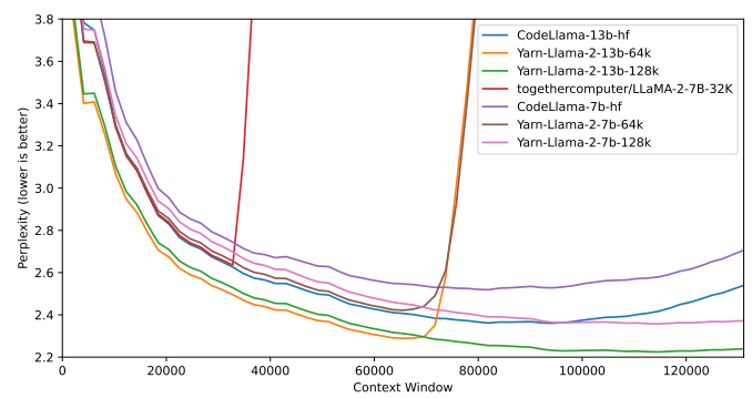
Figure 1: Sliding window perplexity (S = 256) of ten 128k Proof-pile documents truncated to evaluation context window size

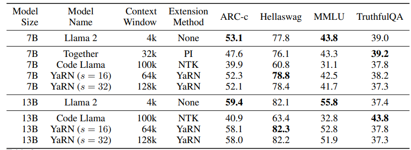
Table 3: Performance of context window extensions methods on the Hugging Face Open LLM benchmark suite compared with original Llama 2 baselines

7. State Space Models (Mamba)

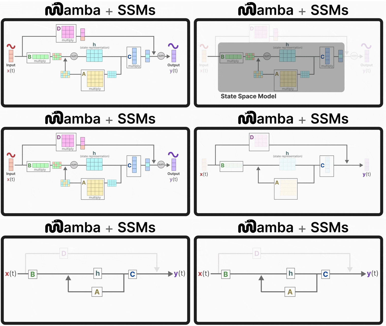
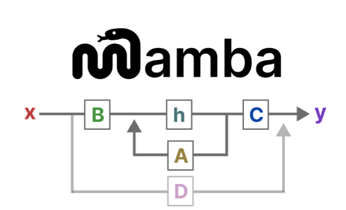
Modern AI language models have long faced a fundamental trade-off, best illustrated by two classic architectures.

7.1 The Transformer: Powerful but Inefficient

The magic of Transformers is self-attention. For any given word, it can directly look at and weigh the importance of every single word that came before it.

• The Blessing (Training): This is highly parallelizable. The attention score between “The” and “cat” can be calculated at the same time as the score between “cat” and “sat.” This makes training on massive GPUs incredibly fast.
• The Curse (Inference): When generating text one word at a time, this becomes a huge bottleneck. To generate the 101st word, the model has to recalculate the attention scores over all 100 previous words. This computational cost grows quadratically (O(N²)). Doubling the text length quadruples the work, making inference for long sequences painfully slow.

7.2 The Recurrent Neural Network (RNN): Efficient but Forgetful

RNNs work sequentially. To process the next word, an RNN only needs two things: the word itself and a compact “hidden state” summarising everything it has seen before.

• The Blessing (Inference): This is incredibly fast and efficient. The computation scales linearly (O(N)). To generate the 101st word, it just updates the state from word 100. The context length is theoretically infinite.
• The Curse (Training & Memory): This sequential nature is slow to train on parallel GPUs. More importantly, RNNs suffer from the “vanishing gradient” problem. Their compressed hidden state tends to forget information from the distant past, making them struggle with long-range dependencies.

So we have a dilemma: Transformers have great memory but slow inference. RNNs have fast inference but poor memory. Can we get the best of both?

7.3 State Space Models (SSMs)

This is where State Space Models (SSMs) enter. Originating from control theory, they offer a powerful way to model sequences. An SSM works just like an RNN: it maintains a hidden state h that gets updated at each step by a new input x.

The core of a classic SSM is defined by two simple linear equations:

ht=Aht−1+Bxtht​=Aht−1​+Bxt​
yt=Chtyt​=Cht​

Let’s assign roles to these matrices:

• h: The hidden state (the model’s “memory”).
• x: The input token.
• y: The output prediction.
• A: The Dynamics Matrix. It defines how the memory h evolves on its own, from one step to the next.
• B: The Input Matrix. It defines how the new input x influences the memory.
• C: The Output Matrix. It defines how the memory h is translated into the final output y.

The S4 “Switcheroo” Trick

Early SSMs (like the S4 model) introduced a brilliant trick. While the equations above look recurrent (and thus slow to train), they can be mathematically transformed into a convolutional form.

1. For Training (Convolutional Mode): The model operates like a CNN. It can process the entire sequence in parallel, making it extremely fast on GPUs.
2. For Inference (Recurrent Mode): It switches back to the recurrent equations shown above, giving it the blazingly fast, linear-time inference of an RNN.

This gave us the best of both worlds in terms of speed. But there was still a critical flaw.

The matrices A, B, and C are fixed. They are learned during training but are the same for every single token at inference time. This property is called Linear Time Invariance (LTI). The model is not content-aware. It can’t change its internal rules based on the data it’s seeing. This means it fails at simple tasks, like selectively copying text, because it can’t “decide” to focus on one piece of information and ignore another.

7.4 Mamba’s Innovations

Mamba solves this final, critical problem with two key innovations.

Innovation 1: The Selection Mechanism

Mamba breaks the chains of LTI. It makes the model content-aware by making the B and C matrices (and a new step-size parameter Δ) dynamic.

Instead of being fixed, B, C, and Δ are now functions of the input token x.

This is the secret sauce.

• If the model sees an important word (e.g., a person’s name), it can generate a B matrix that lets a lot of that information into the hidden state h.
• If it sees a filler word (e.g., “the”), it can generate a B that effectively ignores it, preserving the existing state.
• Similarly, a dynamic C matrix allows it to decide which parts of its memory are relevant for making the next prediction.

This selection ability allows Mamba to compress the sequence’s history intelligently, keeping what’s important and discarding what’s not, much like the attention mechanism in Transformers.

7.5 Hardware-Aware Parallel Algorithm

But wait. If B and C are now dynamic, the neat “convolutional trick” for fast parallel training no longer works! The convolutional kernel would have to change at every single step, defeating the purpose. We seem to be stuck with a slow, recurrent model again.

This is where Mamba’s second breakthrough comes in. The authors designed a hardware-aware algorithm that leverages the memory hierarchy of modern GPUs (SRAM vs. DRAM).

Instead of convolution, it uses a parallel scan. A scan is a classic computer science operation (think “cumulative sum”). While it seems inherently sequential, there are clever parallel algorithms to compute it very quickly. Mamba adapts this to its state calculation.

Furthermore, it uses kernel fusion. Instead of performing multiple steps and writing the intermediate results back to slow global memory (DRAM), it fuses these operations into a single GPU kernel. This minimises memory I/O, which is often the real bottleneck, and dramatically speeds up the process.

7.6 The Mamba Block

Putting it all together, the Mamba architecture consists of:

1. A Selective SSM Core (S6): An SSM that uses the selection mechanism (dynamic B, C, Δ) and is implemented with the fast, hardware-aware parallel scan.
2. HiPPO Initialisation: The crucial A matrix is still initialised using a clever technique called HiPPO, which primes it to be exceptionally good at remembering information over long distances.
3. A Mamba Block: This core S6 layer is wrapped in a block structure very similar to a Transformer block, complete with normalisation and skip connections, allowing them to be stacked deep.

By combining the linear-time efficiency of RNNs with a content-aware selection mechanism that rivals Transformer attention, and then engineering it all to run efficiently on modern hardware, Mamba presents a compelling new foundation for sequence modelling.

8. Vision Language Models (VLLMs)

Vision Language Models (VLMs) are a revolutionary type of generative, multimodal AI that can process and understand both images and text simultaneously. They take visual and textual data as input to generate insightful, text-based outputs. A key strength of modern VLMs is their powerful zero-shot capability, allowing them to perform tasks on new types of images (including documents and web pages) without specific training.

8.1. The Foundational Idea: Teaching a Language Model to See

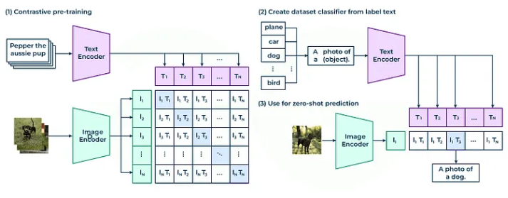
The core challenge in creating VLMs was to represent images and words in a unified mathematical language. The breakthrough was the creation of a shared embedding space, where both visual and textual information could be mapped and compared.

• CLIP (Contrastive Language-Image Pre-training): Developed by OpenAI, CLIP was the model that successfully bridged this gap.
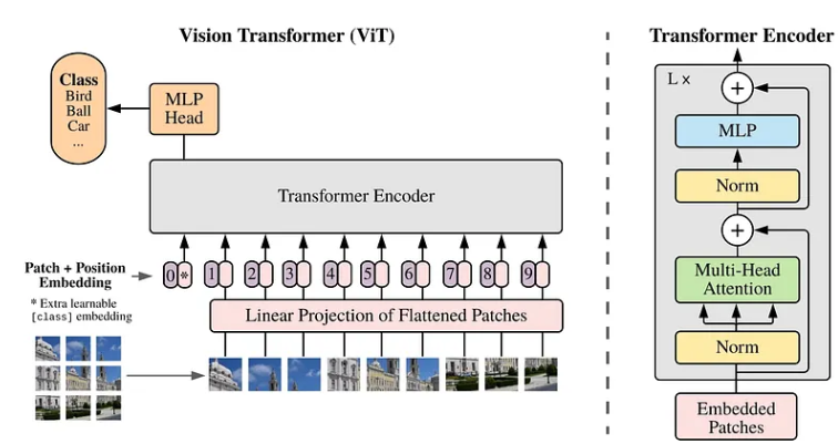
• Architecture: It used two separate neural networks: a Vision Transformer (ViT) for images and a Text Transformer for text.
• Training: It was trained on millions of image-text pairs from the internet. By repeatedly seeing an image of a “dog” with the text “dog,” it learned to associate visual concepts with their descriptions.
• Mechanism: CLIP projects both the image and the text into the same vector space. This allows the model to measure the similarity between an image and a piece of text, forming the foundation for modern generative VLMs.

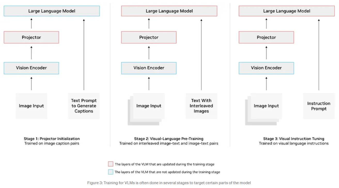
8.2. How a Typical VLM Works: The Three Key Components

Most modern VLMs share a common three-part architecture built on CLIP’s principles:

1. Image Encoder: This is the model’s “eyes.” It uses a Vision Transformer (ViT) to process an image and convert its visual features into a numerical representation (embedding).
2. Multimodal Projector: This acts as a crucial “bridge.” It takes the numerical representation from the image encoder and aligns it into a format that the language model can understand, effectively translating “sight” into “language.”
3. Text Decoder (LLM): This is the model’s “brain.” It’s a Large Language Model that receives the user’s text prompt and the translated visual information, reasoning across both to generate a coherent text response.

8.3. What Can VLMs Do? Applications

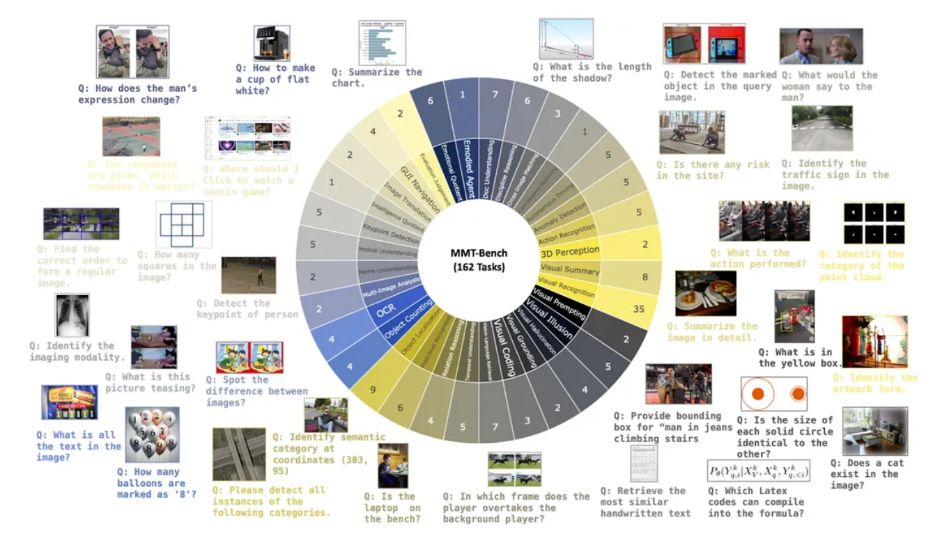
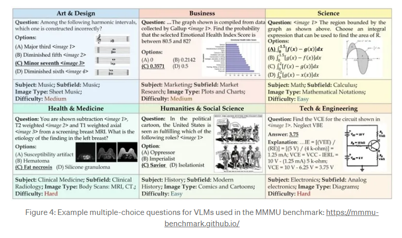
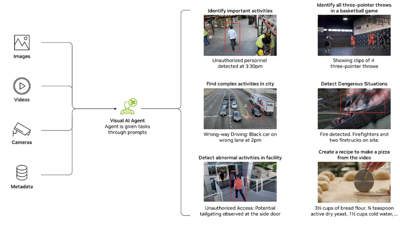
VLMs are transforming technology across various industries with a wide range of applications:

• Image Captioning: Automatically generating descriptive captions, which is vital for accessibility (e.g., screen readers) and content organisation.
• Visual Question Answering (VQA): Answering specific, detailed questions about an image (e.g., “What brand of sneakers is the person wearing?”).
• Image-Text Retrieval: Enhancing search engines by allowing users to search with a combination of an image and a text query (e.g., uploading a photo of a chair and asking, “Where can I buy a similar chair in blue?”).
• Multimodal Assistants: Powering the next generation of AI assistants like GPT-4V, which can understand and respond to both typed text and visual inputs.

8.4. How a VLM ‘Sees’ an Image

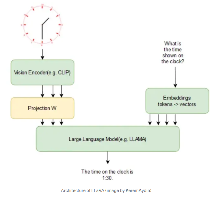
An AI model deconstructs an image into a readable format through a three-step process:

1. The Image Becomes a Sequence of Patches: A Vision Transformer (ViT) splits the image into a grid of small, uniform squares called patches (e.g., 16x16 pixels). The model processes the image as a sequence of these patches.
2. Turning Patches into a Mathematical Language: Each patch is converted into a numerical vector (an embedding) that represents its unique visual information (colour, shape, texture). These vectors are called “visual tokens.”
3. Seeing the Whole Picture with Self-Attention: The model uses a self-attention mechanism to analyse all visual tokens simultaneously, learning the relationships and context between them. This allows it to form a holistic understanding of the entire scene, recognising how different parts of the image relate to one another.

This patch-based approach is revolutionary because it understands context across the entire image and is computationally efficient.

8.5. How VLMs Are Trained

Training a VLM is a multi-stage process to refine its ability to connect vision and language.

• Training Stages:

1. Pretraining: The model learns fundamental connections between images and text by training on massive, web-scale datasets of image-text pairs.
2. Supervised Fine-Tuning (SFT): The model is taught to follow instructions and act as a helpful assistant using a smaller, high-quality dataset of curated examples (e.g., image + question + correct answer).
3. Parameter-Efficient Fine-Tuning (PEFT): A pre-trained VLM is adapted for a specialised domain (e.g., medical imaging) without retraining the entire model, saving time and resources.

Newer Alignment Techniques:

• Direct Preference Optimisation (DPO): An alternative to SFT, DPO fine-tunes a model using preference data. It learns by comparing pairs of responses (“chosen” vs. “rejected”) to generate outputs that align better with human preferences. The RLAIF-V dataset is an example used for this purpose.

8.6. Benchmarking VLMs: Measuring Success

To objectively measure and compare VLM capabilities, researchers use standardised benchmarks.

• Key Benchmarks: MMMU (college-level reasoning), MathVista (math reasoning), and DocVQA (document understanding).
• More Recent Benchmarks: MMT-Bench and MMMU-Pro were developed to provide more complex challenges after some models saturated the initial benchmarks.

8.7. Datasets for Training VLMs

High-quality, aligned multimodal data is crucial for training VLMs.

• LAION-5B: Over 5 billion image-text pairs from the web, supporting multilingual training.
• PMD (Public Model Dataset): Contains 70 billion image-text pairs.
• VQA (Visual Question Answering): Over 200,000 images with questions and answers for fine-tuning reasoning.
• ImageNet: Over 14 million labelled images, primarily for classification and object recognition tasks.

8.8. Current Challenges and Limitations

VLMs still face significant hurdles:

• Technical Hurdles:
• Resolution: Many models struggle with fine details in high-resolution images.
• Spatial Understanding: Models often have difficulty with precise object localisation and spatial relationships (e.g., “to the left of”).
• Long-Context Video: Analysing long videos is computationally expensive and challenging.

Conceptual and Ethical Issues:

• Hallucinations: Generating incorrect information with confidence.
• Inherited Bias: Perpetuating societal biases learned from unfiltered internet data.
• High Computational Cost: Training and deployment require massive resources.
• Ethical Data Sourcing: Concerns over copyright and user consent with web-scraped data.

8.9. Recent Developments and Specialised Capabilities

The VLM field is rapidly advancing with new architectures and specialised models.

• Any-to-Any Models: Can take any modality (image, text, audio) as input and generate output in any modality. Examples include Qwen3-Omni and Chameleon.
• Reasoning Models: Designed for complex problem-solving. Kimi-VL-Thinking is a key example.
• Small Models: Models under 2B parameters (e.g., SmolVLM, Gemma 3) that can run on consumer devices, reducing costs and enhancing privacy.
• Mixture-of-Experts (MoE) Decoders: Architectures that activate only relevant “expert” sub-models for faster, more efficient inference. Llama 4 is a notable example.
• Vision-Language-Action (VLA) Models: VLMs for robotics that generate action tokens to control physical systems. Examples include π0 and GR00T N1.
• Object Detection and Segmentation: Models like PaliGemma and Qwen3-VL can perform traditional computer vision tasks by outputting bounding box coordinates or segmentation masks as text tokens.
• Multimodal Safety Models: Used to filter harmful or inappropriate inputs and outputs. ShieldGemma 2 and Llama Guard 4 are examples.
• Multimodal RAG (Retrieval-Augmented Generation): Enhancing RAG for complex documents (like PDFs) by using multimodal retrievers to find relevant pages, bypassing brittle text parsing.
• Multimodal Agents: VLMs that can understand and operate user interfaces (UIs) for tasks like browser navigation or gameplay. The smolagents library facilitates building such agents.
• Video Language Models: Specialised models that can handle the temporal relationships in videos using techniques like intelligent frame selection (LongVU) or handling dynamic frame rates (Qwen3-VL).

For more details about Vision Language Models (VLMs) from here:

[embed]Vision Language Models (VLMs) An Introduction to how Large Language Models see and understand the world.cbarkinozer.medium.com

9. Quantisation Types

Quantisation as a concept is not new, but the field has evolved rapidly with the rise of Large Language Models. New techniques are constantly being developed to make these massive models more accessible without catastrophic losses in performance. This section breaks down the key quantisation types you will encounter in the Hugging Face ecosystem and beyond, from foundational methods to cutting-edge research.

9.1 Quantisation

Quantisation is a compression technique that involves mapping high-precision values to a lower precision one. For an LLM, that means modifying the precision of their weights and activations, making it less memory-intensive. This surely does have an impact on the capabilities of the model, including the accuracy.

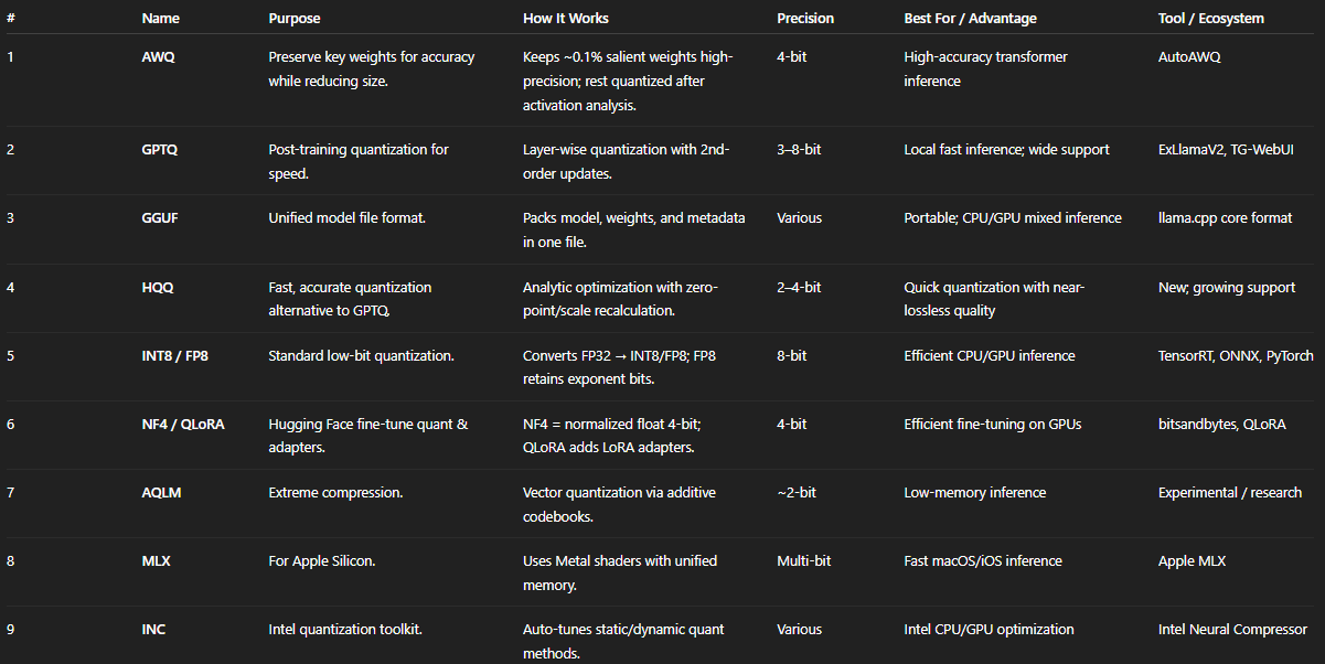
You can find in text format below:

+----+-----------+----------------------------------+---------------------------------------------+-----------+----------------------------------------+----------------------------+
| #  | Name      | Purpose                          | How It Works                                | Precision | Best For / Advantage                   | Tool / Ecosystem           |
+----+-----------+----------------------------------+---------------------------------------------+-----------+----------------------------------------+----------------------------+
| 1  | AWQ       | Preserve key weights for accuracy| Keeps ~0.1% salient weights high-prec, rest | 4-bit     | High-acc transformer inference         | AutoAWQ                    |
|    |           | while reducing size.             | quantised after activation analysis.        |           |                                        |                            |
+----+-----------+----------------------------------+---------------------------------------------+-----------+----------------------------------------+----------------------------+
| 2  | GPTQ      | Post-training quant for speed.   | Layer-wise quant with 2nd-order updates.    | 3–8-bit   | Local fast inference, wide support.    | ExLlamaV2, TG-WebUI        |
+----+-----------+----------------------------------+---------------------------------------------+-----------+----------------------------------------+----------------------------+
| 3  | GGUF      | Unified model file format.       | Packs model + weights + meta in one file.   | Various   | Portable; CPU/GPU mix inference.       | llama.cpp core format      |
+----+-----------+----------------------------------+---------------------------------------------+-----------+----------------------------------------+----------------------------+
| 4  | HQQ       | Fast accurate quant alt to GPTQ. | Analytic opt. with zero-point/scale recalc. | 2–4-bit   | Quick quant with near-lossless quality.| New; growing support       |
+----+-----------+----------------------------------+---------------------------------------------+-----------+----------------------------------------+----------------------------+
| 5  | INT8/FP8  | Standard low-bit quant.          | Converts FP32→INT8/FP8; FP8 keeps exponent. | 8-bit     | Efficient CPU/GPU inference.           | TensorRT, ONNX, PyTorch    |
+----+-----------+----------------------------------+---------------------------------------------+-----------+----------------------------------------+----------------------------+
| 6  | NF4/QLoRA | HF fine-tune quant & adapters.   | NF4 = norm. float 4-bit; QLoRA adds LoRA.   | 4-bit     | Efficient fine-tune on GPUs.           | bitsandbytes, QLoRA        |
+----+-----------+----------------------------------+---------------------------------------------+-----------+----------------------------------------+----------------------------+
| 7  | AQLM      | Extreme compression.             | Vector quant via additive codebooks.        | ~2-bit    | Low-memory inference.                  | Experimental / research    |
+----+-----------+----------------------------------+---------------------------------------------+-----------+----------------------------------------+----------------------------+
| 8  | MLX       | For Apple Silicon.               | Uses Metal shaders + unified memory.        | Multi-bit | Fast macOS/iOS inference.              | Apple MLX                  |
+----+-----------+----------------------------------+---------------------------------------------+-----------+----------------------------------------+----------------------------+
| 9  | INC       | Intel quant toolkit.             | Auto-tunes static/dynamic quant methods.    | Various   | Intel CPU/GPU optimisation.            | Intel Neural Compressor    |
+----+-----------+----------------------------------+---------------------------------------------+-----------+----------------------------------------+----------------------------+

9.2 Core Quantisation Methods & Formats

These are the most common and widely supported quantisation schemes you’ll see used for model deployment.

9.2.1. AWQ (Activation-aware Weight Quantisation)

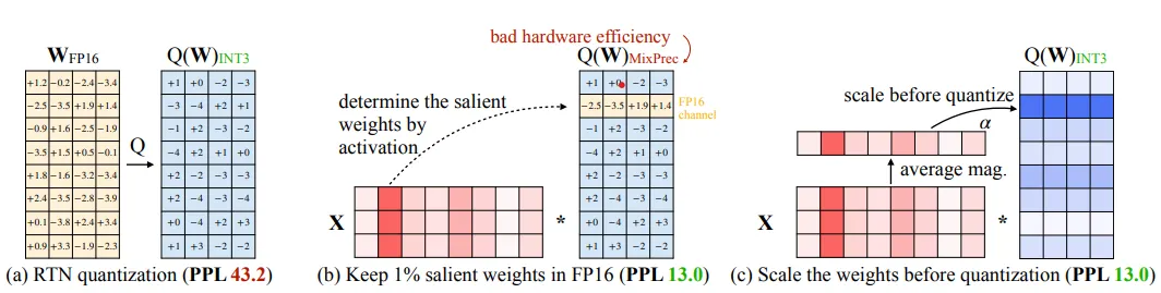
• Purpose: To quantise weights while protecting the most important “salient” weights that have a large impact on the model’s performance. This maintains high accuracy while significantly reducing model size and compute requirements.
• How it works: AWQ observes activations during a calibration step and identifies that a small fraction of weights (around 0.1%) are disproportionately important. It preserves these weights in higher precision and quantises the rest, minimising the impact of activation outliers that harm performance in other methods.
• Precision: Typically 4-bit.
• Best for: Quantising transformer models (e.g., LLaMA, Mistral) for inference with minimal accuracy loss. It often outperforms GPTQ on perplexity benchmarks.
• Tooling: AutoAWQ is the primary library for applying this method.

9.2.2. GPTQ (Post-Training Quantisation for GPT)

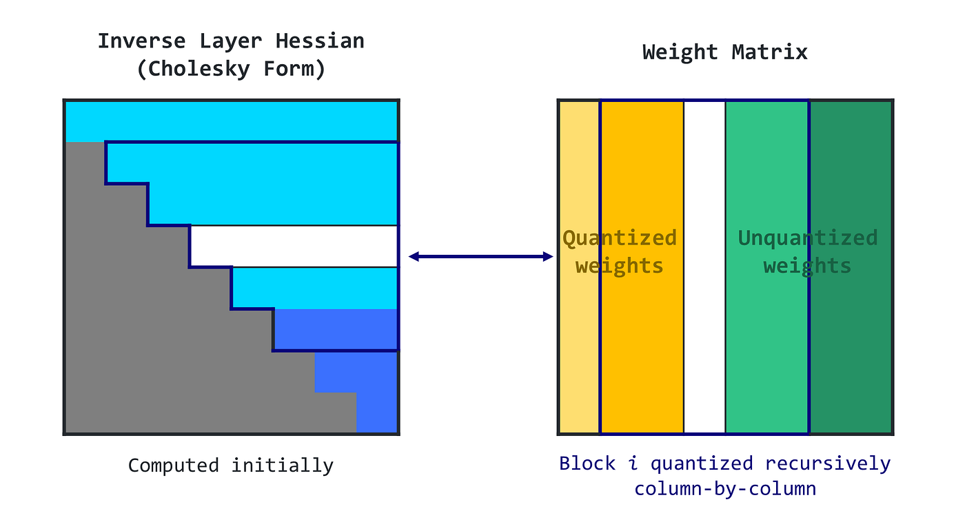
• Purpose: To quantise large models post-training, making inference faster and more memory-efficient with a reasonable trade-off in accuracy.
• How it works: GPTQ iteratively quantises weights layer-by-layer, using a second-order approximation to update the remaining weights to compensate for the error introduced by quantisation. This process requires a small calibration dataset.
• Precision: Typically 4-bit, but can support 3-bit or 8-bit.
• Best for: Running models locally on consumer hardware. It has a mature ecosystem with highly optimised inference kernels like ExLlamaV2.
• Trade-off: Can sometimes be slightly less accurate than AWQ, but is more mature and widely supported across different UIs and backends (e.g., text-generation-webui).

9.2.3. GGUF (GPT-General Unified Format)

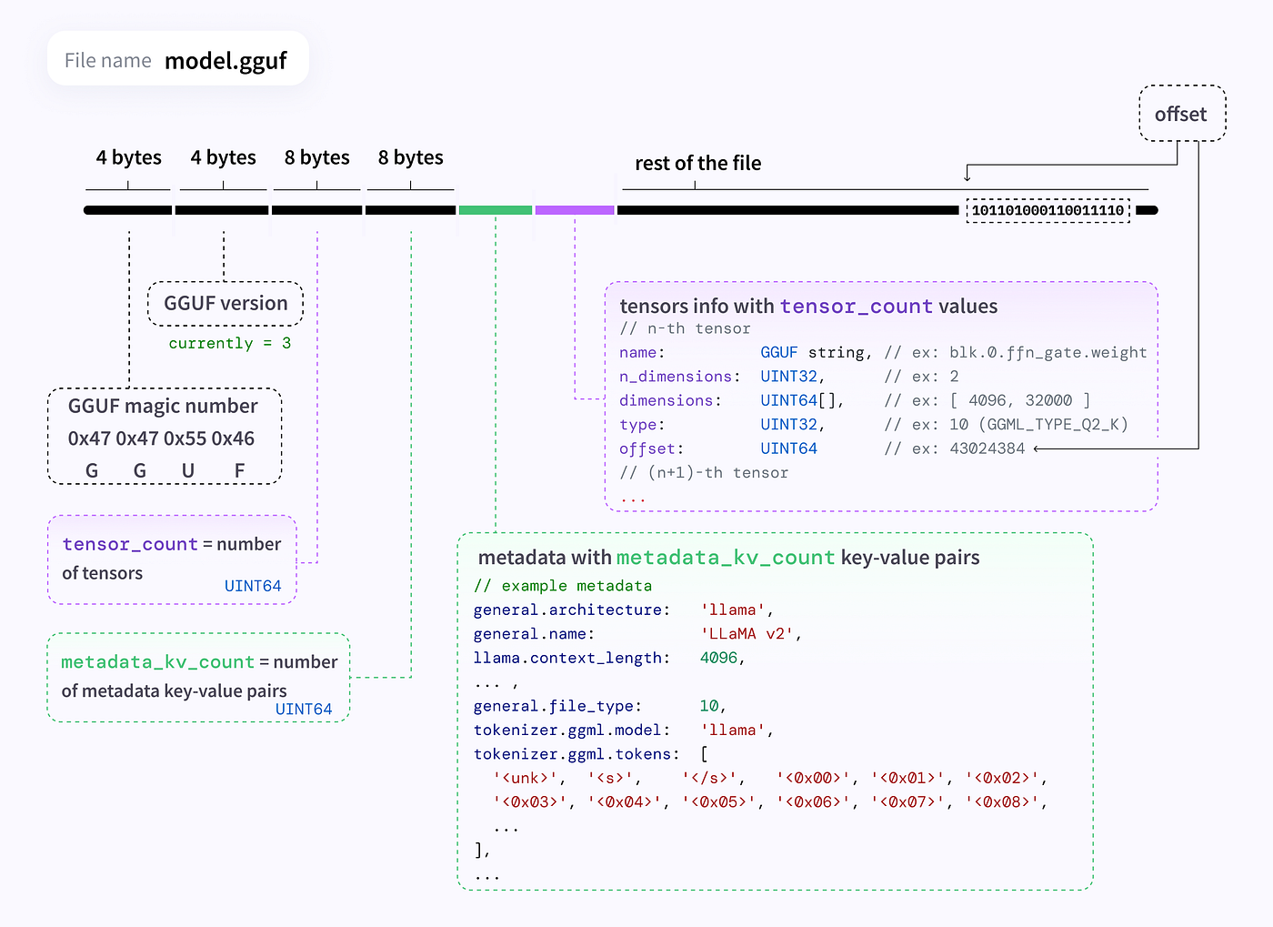
• Purpose: A file format designed for fast loading and efficient inference, primarily on CPUs but with excellent GPU offloading support. GGUF is a container, not a quantisation algorithm itself, but it packages models quantised with various methods.
• How it works: As the successor to the older GGML format, GGUF is a single-file format that includes the model architecture, metadata, and weights. This makes it incredibly portable and easy to use. It supports a wide array of quantisation schemes.
• Quantisation Options: Offers a huge range of schemes, often denoted by Q followed by a number (e.g., Q4_K_M, Q5_K_S, Q8_0). More advanced schemes like IQ (Importance Matrix) Quantisation are also being integrated to improve the accuracy of lower-bit quants.
• Advantages:
• Portability: Single file that works across platforms (Windows, Mac, Linux).
• Flexibility: Allows a mix of CPU and GPU inference.
• Rich Ecosystem: The core of the llama.cpp project, with bindings for many programming languages.

Q4_0 vs Q4_1 vs IQ4_NL

In short, older approaches: Q4_0 is the simplest and least accurate, Q4_1 adds an offset for better representation. A newer approach, IQ4_NL, uses adaptive scaling and importance weighting for much higher accuracy with the same bit size.

Q4_0, Q4_1, and IQ4_NL are all 4-bit quantisation formats, meaning each model weight is stored using just 4 bits instead of 16 or 32. This greatly reduces memory use and speeds up inference.

In Q4_0, weights are grouped into small blocks of 32 values. Each block has one scale factor that rescales the 4-bit integers (q) back into approximate real numbers using the formula w = q × block_scale. Since it has no offset, it assumes the weights are roughly centred around zero, which can reduce accuracy if they aren’t.

Q4_1 improves this by adding a block_minimum value (an offset) to the formula: w = q × block_scale + block_minimum. This lets it represent asymmetric weight distributions better — for example, when all weights in a block are positive. The quantisation is still done per 32-weight block, so it’s simple but not very flexible.

IQ4_NL (Improved Quantisation 4-bit, Non-Linear) is a newer and more advanced approach. It groups weights into super-blocks of 256 weights and applies a more complex scaling strategy using a super_block_scale and an importance matrix. The importance matrix adjusts scaling based on how important each subset of weights is to model accuracy. This allows the quantisation to preserve more detail in critical weights while still using only 4 bits per value.

9.2.4. HQQ (Half-Quadratic Quantisation)

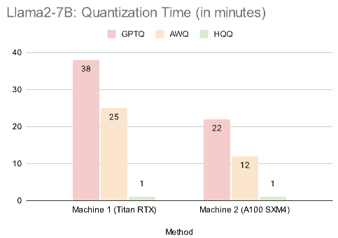
• Purpose: An extremely fast and accurate post-training quantisation method that often matches the performance of GPTQ and AWQ with significantly faster quantisation times.
• How it works: HQQ models quantisation as an optimisation problem that can be solved analytically without slow, iterative updates. This results in a “lossless” compression from a theoretical standpoint, as the dequantization process uses a zero-point and scale that perfectly reconstructs the original weight matrix’s properties.
• Precision: Supports 4-bit, 3-bit, and even 2-bit quantisation.
• Best for: Rapidly quantising models with excellent performance, serving as a strong and fast alternative to GPTQ/AWQ.
• Trade-off: A newer method, so ecosystem support is still growing compared to the more established formats.

Foundational Concepts & Tooling

These entries describe either fundamental building blocks or overarching frameworks for quantisation.

9.2.5. INT8 / FP8 Quantisation (Standard Quantisation)

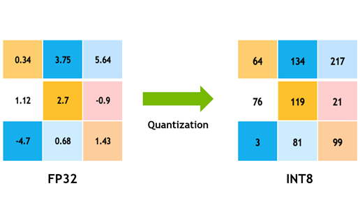
• What it is: The “classic” form of quantisation. Instead of using 32-bit or 16-bit floating-point numbers, weights and/or activations are converted to 8-bit integers (INT8) or 8-bit floats (FP8).
• INT8: Offers fast computation on modern CPUs and GPUs but can struggle with the wide dynamic range of values in LLMs, leading to accuracy loss.
• FP8: A newer format supported by modern GPUs (NVIDIA H100 and newer) that retains the exponent bits, making it much better at handling outliers and maintaining accuracy.
• Tooling: A standard feature in deep learning compilers and runtimes like NVIDIA TensorRT, ONNX Runtime, and PyTorch (which uses backends like fbgemm for efficient INT8 CPU operations).

9.2.6. Hugging Face bitsandbytes Integration (NF4 & QLoRA)

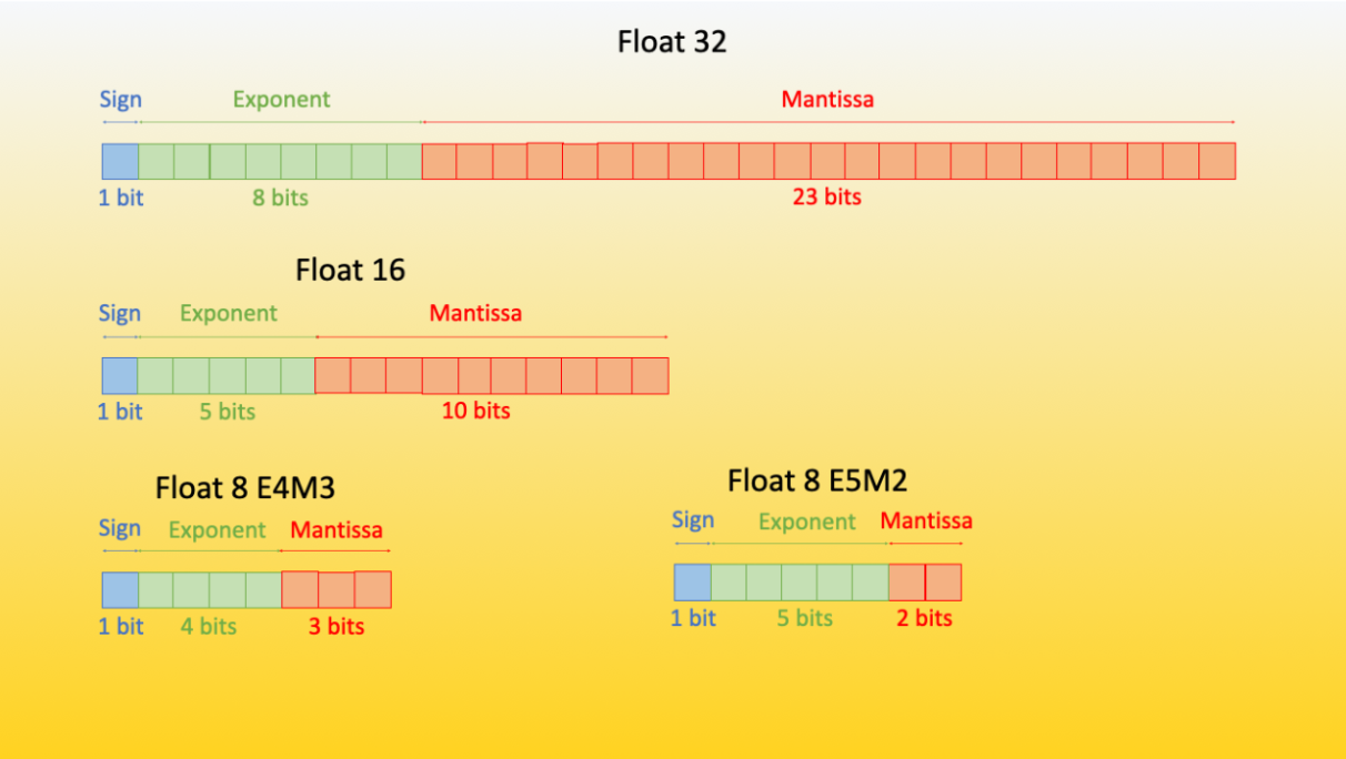
• What it is: The bitsandbytes library is a cornerstone of Hugging Face’s native quantisation, enabling on-the-fly quantisation during model loading.
• NF4 (Normalised Float 4-bit): A special 4-bit data type superior to standard 4-bit integers. It’s designed based on the observation that neural network weights are typically normally distributed. NF4 has more precision points clustered around zero, which better preserves the original weight distribution.
• QLoRA: A revolutionary technique for efficient fine-tuning. It works by:

1. Quantising a pre-trained base model to 4-bit using NF4.
2. Freezing these quantised weights.
3. Attaching and training small LoRA (Low-Rank Adaptation) adapters in 16-bit precision.

• This dramatically reduces the memory required for fine-tuning, allowing massive models to be trained on consumer GPUs.

9.2.7. AQLM (Additive Quantisation of Language Models)

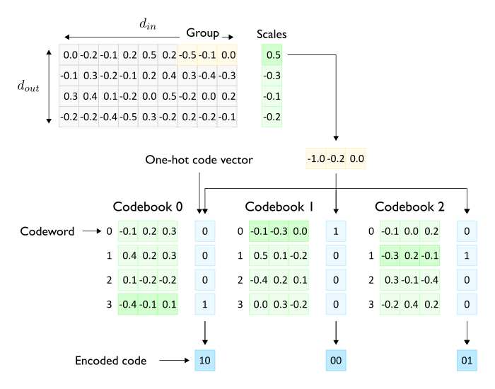
• Purpose: An advanced quantisation method designed for extreme compression, enabling models to run at very low bitrates (e.g., 2-bit) with surprisingly good performance.
• How it works: Instead of quantising each weight individually, AQLM uses vector quantisation. It groups weights into vectors and represents each vector with a code from a learned “codebook.” The final representation is a sum of a few codebook entries, allowing for high compression with better accuracy than naive 2-bit methods.
• Best for: Scenarios where memory and bandwidth are severely constrained, and a moderate perplexity trade-off is acceptable.

9.2.8. MLX (Apple MLX Quantisation)

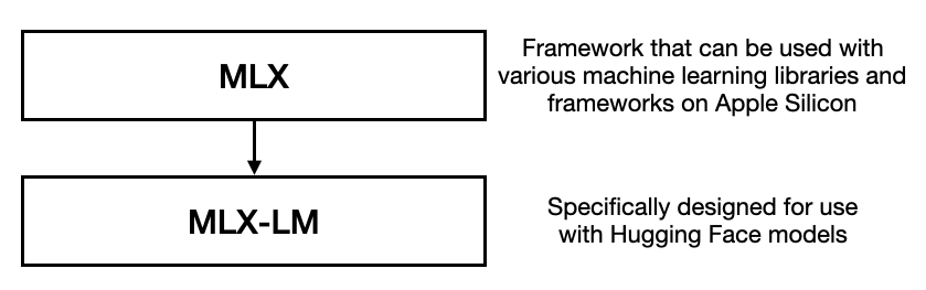
• Purpose: Apple’s native framework for running and quantising models efficiently on Apple Silicon (M1/M2/M3/M4 chips).
• How it works: MLX leverages Apple’s unified memory architecture and Metal Performance Shaders for hardware-accelerated inference. Its quantisation utilities are optimised specifically for this stack.
• Key Features:
• Native Acceleration: The fastest way to run LLMs on macOS and iOS.
• Simplified API: Easy-to-use Python API for loading, quantising, and running models.
• Use Case: The go-to solution for anyone developing or running LLMs on Apple hardware.

9.2.9. Intel® Neural Compressor (INC)

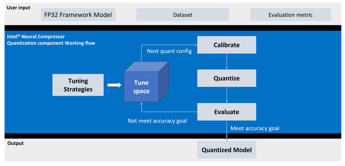
• Purpose: A powerful toolkit from Intel for optimising deep learning models for inference on Intel hardware (CPUs, GPUs).
• How it works: INC is a framework that automates the optimisation process. It supports various quantisation algorithms (static, dynamic, GPTQ-like) and features an automatic tuning engine that searches for the optimal quantisation strategy to meet a user-defined accuracy goal.
• Best for: Deploying models in production environments on Intel servers or client devices where performance and efficiency are critical.

10. Reinforcement Learning From Human Feedback (RLHF)

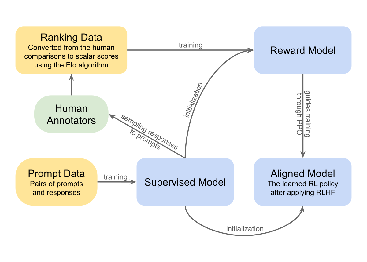
Language models (LMs) have demonstrated impressive capabilities by generating diverse and compelling text from human prompts. However, the standard pretraining method, which uses a simple next-token prediction loss (e.g., cross-entropy), is insufficient to capture what makes text “good,” a quality that is inherently subjective and context-dependent. Metrics like BLEU and ROUGE were developed to better measure human preferences but are limited by their simple, rule-based comparisons to reference texts.

Even after a large language model (LLM) is pretrained on massive text corpora and fine-tuned on curated instruction datasets, it still doesn’t fully grasp human preferences. Reinforcement Learning from Human Feedback (RLHF) is the crucial final alignment stage that makes models like ChatGPT and Claude feel natural, polite, and helpful. The core idea of RLHF is to use direct human feedback not just as a performance metric but as a loss signal to optimise the model, thereby aligning it with complex human values and expectations.

10.1 The Three Core Steps of the RLHF Process

RLHF is a challenging, multi-model training process that combines machine learning with human judgment. It unfolds in three key steps:

1. Pretraining a Language Model (LM)

The process begins with a language model that has already been pretrained using classical objectives. There is no single “best” starting model, and different organisations have used models of varying scales:

• OpenAI used a smaller version of GPT-3 for InstructGPT.
• Anthropic has used models ranging from 10M to 52B parameters.
• DeepMind has used its 280B parameter Gopher model.

Optionally, this base model can be further fine-tuned on a small, high-quality dataset of human-generated text to improve its ability to follow instructions before the main RLHF process begins. The key requirement is to start with a model that responds well to diverse prompts.

2. Gathering Human Preference Data and Training a Reward Model (RM)

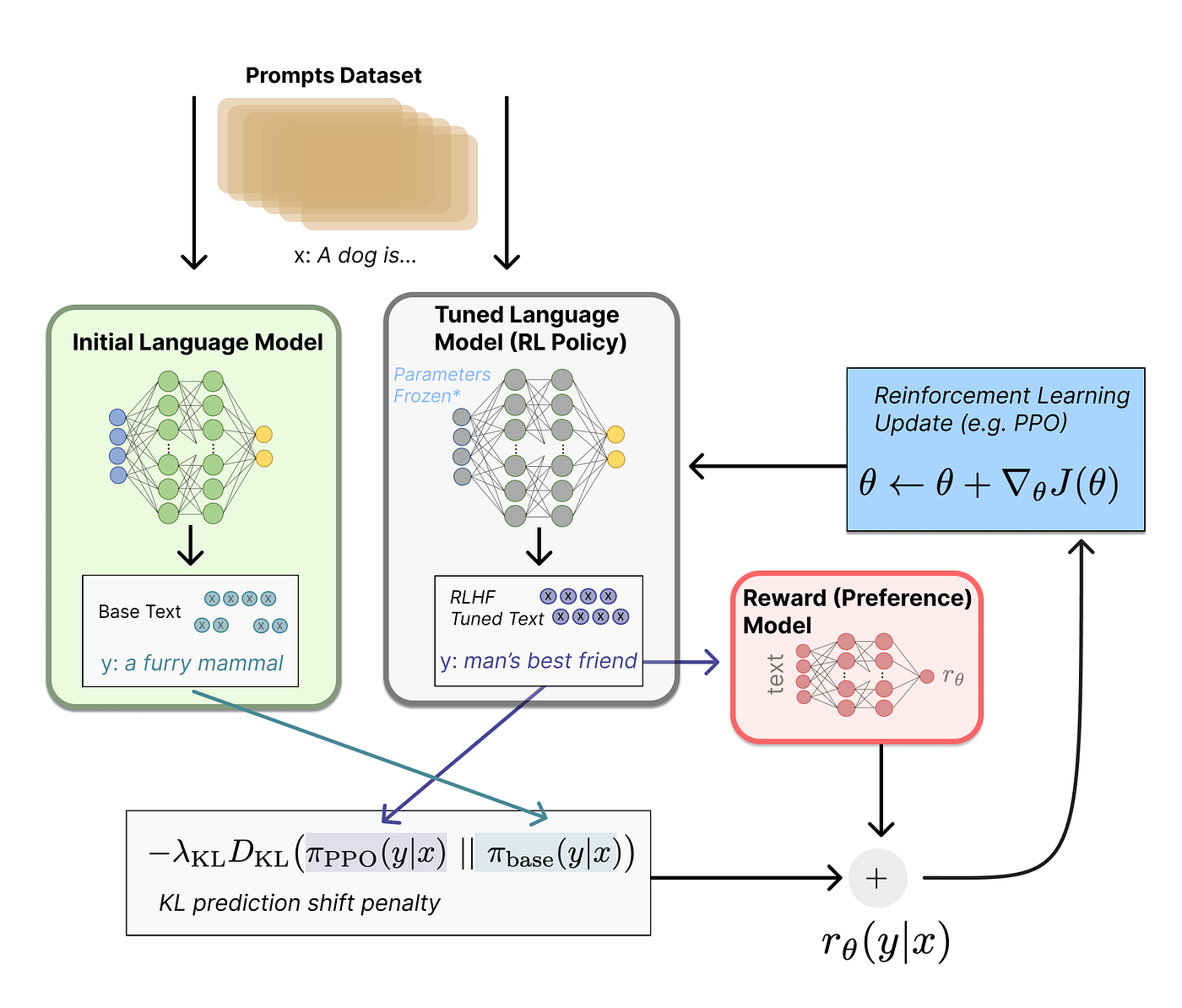
This step is where human preferences are formally integrated. The goal is to create a reward model (RM) that can predict these preferences.

• Collect Human Preferences: First, a set of prompts is sampled. The initial LM generates two or more responses for each prompt. Human labellers are then shown these pairs of responses and asked to choose which one they prefer. These comparisons capture subjective qualities like helpfulness, accuracy, tone, and safety. Using rankings or comparisons is more effective than asking for direct scalar scores, as it produces a better-regularised and less noisy dataset. An Elo rating system can be used to rank outputs from head-to-head matchups.
• Train a Reward Model: This collected preference data is used to train a separate model — the reward model. The RM takes any text sequence as input and assigns a single scalar “reward score” to it, effectively quantifying how much a human would likely prefer that output. The RM can be another fine-tuned LM or one trained from scratch. Interestingly, successful RMs have often been significantly smaller than the LMs they evaluate (e.g., OpenAI’s 175B LM and 6B RM).

3. Fine-tuning the LLM with Reinforcement Learning (RL)

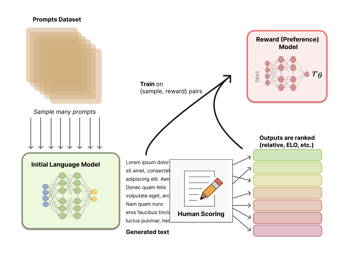
In the final step, the base LLM is optimised using RL to maximise the reward signal from the RM.

• RL Formulation: The LLM acts as the policy, which takes a prompt and generates text. The action space is the model’s vocabulary (~50k tokens), and the observation space is the distribution of possible input prompts.
• Reward Function: The total reward is a combination of two signals:

1. Preference Score (rθrθ): The score from the reward model for the generated text.
2. KL Divergence Penalty (rKL*rKL*​): To prevent the model from deviating too far from the original pretrained model and generating incoherent text that “hacks” the reward system, a penalty is applied. This is typically a scaled Kullback-Leibler (KL) divergence between the token distributions of the current policy and the initial, frozen model. The final reward is:r=rθ−λrKL*r*=*rθ*​−*λrKL.*​

Optimisation Algorithm: The most common algorithm used is Proximal Policy Optimisation (PPO), a mature policy-gradient method. Due to the immense cost of updating a full LLM, often only a subset of the parameters is fine-tuned (e.g., using techniques like LoRA).

This process can also be iterative. As the policy improves, new outputs can be collected and ranked by humans, and both the reward model and the policy can be updated together in a cycle.

The Result: An Aligned Model

Through RLHF, the model transitions from merely predicting the next token to aligning with human values. It learns to:

• Follow nuanced and complex instructions.
• Avoid generating toxic, harmful, or unsafe content.
• Express uncertainty when appropriate.
• Be more conversational, context-aware, and helpful.

10.2 PPO vs DPO

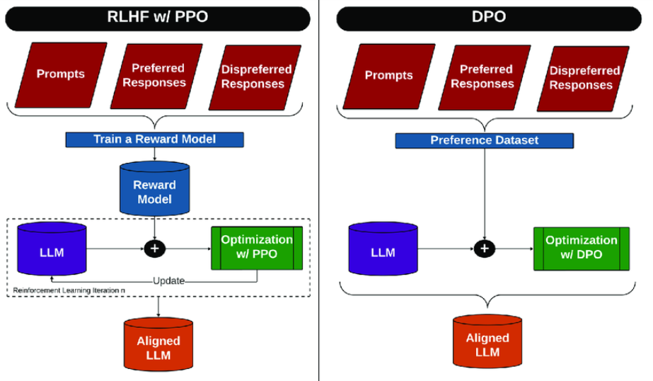
PPO vs DPO

Now that we understand the intricate three-step process of Reinforcement Learning from Human Feedback (RLHF), which often culminates in using Proximal Policy Optimisation (PPO), it’s time to explore a newer, more streamlined approach that has gained significant traction: Direct Preference Optimisation (DPO).

While PPO represents a powerful and thorough method for model alignment, it is notoriously complex and resource-intensive. DPO offers an elegant alternative by reframing the problem. To understand the difference, let’s use an analogy: learning to play chess.

• PPO is like learning with a live coach. You actively play games, and after every move, your coach gives you feedback. You learn by doing, exploring new strategies, and continuously adjusting your play style based on real-time results.
• DPO is like learning from a pre-written chess manual. You study a book filled with examples of game positions, each showing a “winning move” and a “losing move.” You learn by memorising these patterns and internalising the principles of what makes one move better than another, without ever playing a live game during your study session.

This core difference stems from their underlying learning paradigms: On-Policy vs. Off-Policy.

• On-Policy (PPO): The model generates its own training data in real-time. It acts, gets feedback, and learns from its own current behaviour. It’s constantly exploring.
• Off-Policy (DPO): The model learns from a static, pre-collected dataset of preferences (e.g., “Response A is better than Response B”). It doesn’t need to generate anything new during this training phase.

Let’s break down how each approach works and what its trade-offs are.

Understanding PPO: The Live Coaching Method

As we’ve seen, PPO is the final, dynamic stage of the classic RLHF pipeline. It requires a whole team of models working together:

1. The Actor: The language model we are fine-tuning. It generates responses (“plays the game”).
2. The Reward Model (The Referee): A separate model that scores the Actor’s response, providing a final judgment on its quality.
3. The Critic (The Coach): Often part of the Actor model, this component estimates the potential future rewards from a given point, providing an immediate sense of whether a move was good or bad.
4. The Reference Model (The Rulebook): A frozen copy of the original model, used to ensure the Actor doesn’t stray too far from coherent language in its pursuit of high rewards (this is the KL penalty, or “leash”).

The PPO process is an active loop: the Actor generates a response, the Referee and Critic evaluate it, and the system calculates the advantage, much better or worse than that response was than expected. The Actor’s parameters are then nudged to make responses with a positive advantage more likely. This on-policy, trial-and-error process is powerful because the model learns from its current capabilities, but it is also incredibly computationally expensive, often requiring multiple massive models to be loaded into memory at once.

Understanding DPO: The Chess Manual Method

DPO’s creators realised that the complex PPO loop could be simplified. Through a clever mathematical insight, they found that the end goal of the RLHF process, aligning the model with human preferences, could be achieved directly, without the intermediate steps of training a separate reward model and running a reinforcement learning loop.

Instead of a live coaching session, DPO works like this:

1. Start with the Manual: You begin with a preference dataset. Each entry contains a prompt, a “chosen” (preferred) response, and a “rejected” (disliked) response.
2. Directly Optimise: The DPO algorithm trains the language model with a single, elegant objective: increase the relative probability of the chosen response and decrease the relative probability of the rejected response.

That’s it. No explicit reward model is being trained first, and no complex RL sampling loop. The human preference is translated directly into a loss function that the language model can optimise. It effectively learns the underlying “reward” implicitly by observing the human preferences in the dataset. This makes DPO far simpler, more stable, and much less computationally demanding than PPO.

Key Differences and Limitations

While DPO’s simplicity is appealing, the choice between these two methods involves significant trade-offs.

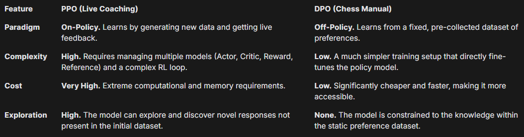
This leads to a crucial limitation of DPO, often called the “Evaluation vs. Generation” Gap.

DPO trains the model to be an excellent judge of responses based on the patterns in the preference data. It learns to recognise what makes one answer better than another. However, it doesn’t get any practice in the act of generation during this phase. There’s a risk that this learned “evaluation skill” doesn’t perfectly translate into generating high-quality responses in the wild. PPO, by its nature, forces the model to both generate and evaluate in a tight loop, inherently closing this gap.

Furthermore, DPO’s performance is entirely dependent on the quality and coverage of its offline dataset. If the preference data is narrow or fails to cover diverse scenarios, the model can learn to exploit its patterns in unexpected ways. For instance, if a model learns only that “tomato sauce” is preferred over “chilli oil” for pasta, it might bizarrely conclude that “concrete grade 42” is an acceptable alternative, as it was never told otherwise. Because PPO is online and exploratory, it is theoretically less susceptible to such out-of-distribution failures.

Conclusion: Which Method to Choose?

Neither PPO nor DPO is universally superior; the best choice depends on the goal.

• PPO remains the heavyweight champion for achieving the absolute highest performance ceiling. Its ability to explore and learn from live feedback makes it ideal for developing state-of-the-art, frontier models where complexity and cost are secondary concerns.
• DPO is the pragmatic and efficient challenger. It has democratized model alignment, allowing researchers and smaller organisations to effectively fine-tune models without the prohibitive costs of PPO. Its simplicity and stability make it an incredibly powerful and popular tool.

Ultimately, both PPO and DPO are milestones in the quest to create AI that is not only capable but also helpful, harmless, and aligned with human values. The field continues to evolve rapidly, with new methods constantly emerging to strike an even better balance between performance, efficiency, and stability.

10.3 Open-Source Tools and Datasets

Several open-source tools facilitate RLHF:

• TRL (Transformers Reinforcement Learning): For fine-tuning Hugging Face models with PPO.
• TRLX: An expanded fork for large-scale models, supporting PPO and ILQL.
• RL4LMs: A highly customizable library with a wide variety of RL algorithms and reward functions. A large-scale dataset created by Anthropic is also publicly available.

10.4 Limitations and Challenges of RLHF

Despite its success, RLHF has clear limitations:

• Performance: Models can still output harmful or factually inaccurate text.
• Data Cost: Gathering high-quality human preference data is expensive and time-consuming, often requiring hired staff rather than crowdsourcing.
• Data Availability: Very few large-scale, general-purpose RLHF datasets exist publicly.
• Annotator Disagreement: Humans often disagree, introducing variance and noise into the training data.

10.5 The Future: Beyond RLHF

The field is actively exploring improvements and alternatives:

• Better RL Optimisers: Researchers are investigating alternatives to PPO, including offline RL algorithms like Implicit Language Q-Learning (ILQL) to reduce the computational cost of the fine-tuning loop.
• Direct Preference Optimisation (DPO) and KTO: Recent innovations such as Direct Preference Optimisation (DPO) and Kullback–Leibler Preference Optimisation (KTO) aim to streamline the alignment process. These methods directly fine-tune models from preference data without needing a separate reward model or an explicit reinforcement learning loop, making alignment simpler, more stable, and more scalable.

References

[1] cbarkinozer, (Aug 5, 2025), MoE: Uzman Karması (Mixture-of-Experts):

[https://medium.com/softtechas/moe-uzman-karmas%C4%B1-mixture-of-experts-ecdc357d3de2]

[2] azhar, (Jan 11, 2024), Rotary Positional Embeddings: A Detailed Look and Comprehensive Understanding

[https://medium.com/ai-insights-cobet/rotary-positional-embeddings-a-detailed-look-and-comprehensive-understanding-4ff66a874d83]

[3] Tri Dao, Daniel Y. Fu, Stefano Ermon, Atri Rudra, Christopher Ré, (23 Jun 2022), FlashAttention: Fast and Memory-Efficient Exact Attention with IO-Awareness

[https://arxiv.org/abs/2205.14135]

[4] huggingface, (2025), Flash Attention

[https://huggingface.co/docs/text-generation-inference/conceptual/flash_attention]

[5] Loïck BOURDOIS, (July 19, 2024), Introduction to State Space Models (SSM)

[https://huggingface.co/blog/lbourdois/get-on-the-ssm-train]

[6] Maarten Grootendorst, (Feb 19, 2024), A Visual Guide to Mamba and State Space Models

[https://newsletter.maartengrootendorst.com/p/a-visual-guide-to-mamba-and-state]

[7] mervenoyan, edbeeching, (April 11, 2024), Vision Language Models Explained

[https://huggingface.co/blog/vlms]

[8] Bordres, Pang, (27 May 2024), An Introduction to Vision-Language Modelling

[https://arxiv.org/abs/2405.17247]

[9] Kerem Aydin, (Feb 29, 2024), What are Visual Language models and how do they work?

[https://medium.com/@aydinKerem/what-are-visual-language-models-and-how-do-they-work-41fad9139d07]

[10] NVIDIA, (2025), What Are Vision Language Models

[https://www.nvidia.com/en-us/glossary/vision-language-models/]

[11] sandeep (June 4, 2025), Introduction to Vision Language Models:

[https://opencv.org/blog/vision-language-models/]

[12] merve, sergiopaniego, ariG23498, pcuenq, andito, (May 12, 2025), Vision Language Models (Better, Faster, Stronger):

[https://huggingface.co/blog/vlms-2025]

[13] Huggingface, (2025), GGUF:

[https://huggingface.co/docs/hub/gguf]

[14] Nathan Lambert, Louis Castricato, Leandro von Werra, Alex Havrilla, (December 9, 2022), Illustrating Reinforcement Learning from Human Feedback (RLHF):

[https://huggingface.co/blog/rlhf]

[15] Yihua Zhang, (February 11, 2025), Navigating the RLHF Landscape: From Policy Gradients to PPO, GAE, and DPO for LLM Alignment:

[https://huggingface.co/blog/NormalUhr/rlhf-pipeline]