Test-Time Scaling Part 1: Foundations and Mechanics

Understanding How LLMs Learn to “Think Longer” During Inference

Introduction: Beyond Training-Time Scaling

For years, the AI community followed a simple mantra: bigger models, more data, more compute. This “scaling law” paradigm, exemplified by GPT-3’s 175 billion parameters and subsequent models, focused almost exclusively on training-time scaling — making models larger and training them on more data.

But in late 2022, a quiet revolution began. Researchers asked a deceptively simple question:

What if we could make models “smarter” not by training them longer, but by letting them “think” longer at inference time?

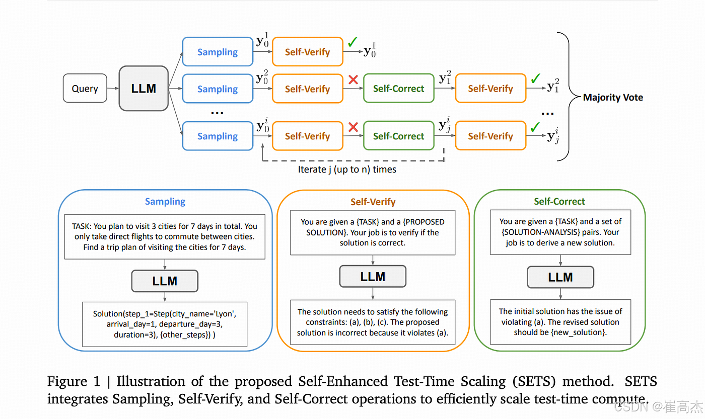
This is test-time scaling (also called inference-time compute scaling): the idea that allocating more computational resources during inference — when the model generates answers — can yield better, more accurate, and more reliable outputs.

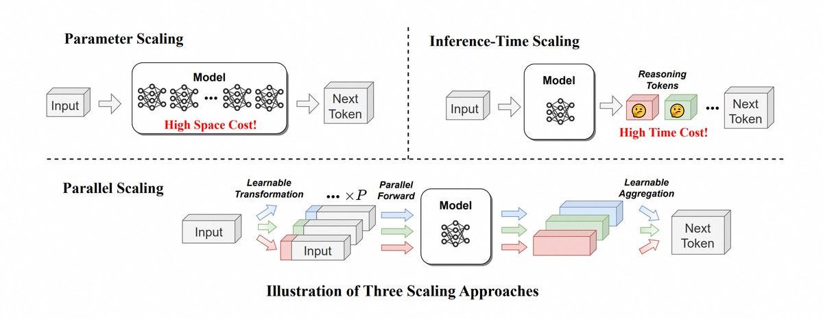
Train Time Scaling vs Test Time Scaling

Important distinction: Test-Time Scaling (TTS) is different from Test-Time Adaptation (TTA). TTS keeps the model weights completely frozen and instead allocates more computational resources (10–100x more) to improve reasoning — using techniques like Chain-of-Thought prompting, self-consistency with multiple samples, Tree of Thoughts search, or Monte Carlo Tree Search to generate and verify multiple solution paths. In contrast, TTA temporarily updates the model’s parameters during inference (via gradient descent) to adapt to distribution shifts or domain changes, using methods like entropy minimization, pseudo-labeling, or self-supervised tasks, while maintaining similar compute cost to standard inference. In essence, Test-Time Scaling = “think longer with the same brain” (fixed model θ, variable compute), while Test-Time Adaptation = “adjust the brain to new environments” (variable model θ → θ’, standard compute). The former tackles complex reasoning problems on the same distribution; the latter handles covariate shift and domain adaptation.

┌─────────────────────────────────────────────────────────────┐
│                  TEST-TIME SCALING                          │
├─────────────────────────────────────────────────────────────┤
│  Model: θ (fixed) - Generate multiple solutions             │
│                   - Extended reasoning (CoT, ToT)           │
│                   - Self-consistency voting                 │
│                   - Search & verification                   │
│                                                             │
│  Compute: 1x → 100x                                         │
│  Parameters: Unchanged                                      │
│  Goal: Better answers via more thinking                     │
└─────────────────────────────────────────────────────────────┘

┌─────────────────────────────────────────────────────────────┐
│                TEST-TIME ADAPTATION                         │
├─────────────────────────────────────────────────────────────┤
│  Model: θ → θ' (adapted) via gradient updates               │
│         - Minimize entropy on test data                     │
│         - Self-supervised auxiliary tasks                   │
│         - Pseudo-labeling                                   │
│                                                             │
│  Compute: ~1x (similar to standard)                         │
│  Parameters: Temporarily updated                            │
│  Goal: Adapt to distribution shift                          │
└─────────────────────────────────────────────────────────────┘

The Core Insight

Traditional inference is a single forward pass:

Input → Model → Output (done in ~1 second)

Test-time scaling transforms this into:

Input → Model thinks (searches, verifies, iterates) → Better Output (done in ~10-60 seconds)

The model uses extra time to:

• Generate multiple candidate answers
• Verify and critique its own outputs
• Search through reasoning paths
• Refine and improve solutions iteratively

Why this matters: While training a 10x larger model might cost millions of dollars and months of time, test-time scaling can achieve comparable improvements by simply running the model longer — a trade-off anyone can make on-demand.

The Historical Context: Why Now?

Pre-2022: Inference Was “Free”

Before large language models (LLMs), inference was trivial:

• Image classification: 10ms per image
• Translation: 100ms per sentence
• Search queries: instant

The computational budget was spent almost entirely on training.

2022–2023: The ChatGPT Shift

ChatGPT changed everything:

1. Inference became expensive: Generating 1000 tokens could cost $0.02–0.10
2. Quality became critical: Users would wait 10–30 seconds for better answers
3. Reasoning emerged: Models could solve complex problems if guided properly

Suddenly, spending more compute at test time became economically viable and desirable.

The Scaling Laws Evolution

Training-time scaling (2018–2022):

Test-time scaling (2022+):

The new dimension: how much you compute during inference.

The Fundamental Scaling Laws

Understanding the Tradeoff

Observation: Test-time compute follows power laws similar to training-time scaling.

Empirical scaling law (from OpenAI, DeepSeek research):

Where:

• N = test-time compute (in FLOPs or tokens)
• A = asymptotic performance
• B, C, α = task-dependent constants

Key insight: Diminishing returns but smooth, predictable scaling.

Cost-Performance Curves

Optimal allocation depends on value of accuracy:

• Research: Use 125x (maximize accuracy)
• Production: Use 5–25x (balance cost/quality)
• Bulk processing: Use 1x (minimize cost)

Training-Time vs Test-Time Scaling Comparison

Optimal strategy: Combine both!

1. Train powerful base model (training-time scaling)
2. Apply test-time scaling as needed for difficult queries

Strategy Comparison by Problem Characteristics

Timeline of different TTS Strategies (Credits:

Different test-time scaling strategies excel at different problem types:

Test Time Scaling Strategies

The Mechanics: How LLMs Generate Multiple Reasoning Steps

Understanding test-time scaling requires understanding how LLMs generate reasoning at a mechanical level.

Token-by-Token Generation Process

At its core, an LLM generates text one token at a time through autoregressive generation:

def generate_text(prompt, model, max_tokens=100):
    tokens = tokenize(prompt)

    for i in range(max_tokens):
        # 1. Embed current tokens
        embeddings = embed(tokens)

        # 2. Run through transformer layers
        hidden_states = model.forward(embeddings)

        # 3. Project to vocabulary space
        logits = hidden_states[-1] @ model.output_projection

        # 4. Sample next token
        probs = softmax(logits / temperature)
        next_token = sample(probs)

        # 5. Append and continue
        tokens.append(next_token)

        if next_token == END_TOKEN:
            break

    return detokenize(tokens)

Key insight: Each forward pass computes the probability distribution for the next token only. The model doesn’t “plan ahead” — it makes local decisions that compound into global behavior.

How Chain-of-Thought Works Mechanically

When we prompt with “Let’s think step by step,” we’re actually changing the probability distribution of generated tokens:

Without CoT prompt:
P("11" | "Roger has 5 balls, buys 2 cans of 3 =") = 0.15 ✓
P("10" | "Roger has 5 balls, buys 2 cans of 3 =") = 0.25 ❌ (wrong but higher!)

With CoT prompt ("Let's think step by step"):
P("Roger starts with" | "Let's think step by step.") = 0.45
P("5 tennis balls" | "Let's think step by step. Roger starts with") = 0.67
...
[After 50 tokens of reasoning]
P("11" | "...Total: 5 + 6 =") = 0.85 ✓ (now higher!)

Why it works:

1. Intermediate tokens provide better context for final answer.
2. Step-by-step structure mirrors human reasoning patterns from training data.
3. More compute (50 tokens vs 5) allows model to “work through” the problem.

Multiple Sampling: Diversity Through Temperature

For techniques like self-consistency, we need diverse reasoning paths:

def sample_with_temperature(logits, temperature=1.0):
    # Higher temperature = more randomness = more diversity
    probs = softmax(logits / temperature)
    token = sample_from_distribution(probs)
    return token

# Example: Sampling next word after "Each apple costs"
logits = [5.2, 4.8, 3.1, ...]  # For tokens ["$2", "$3", "$6", ...]

Temperature = 0.1 (low):
  probs = [0.62, 0.35, 0.02, ...]  # Nearly deterministic

Temperature = 0.7 (medium):
  probs = [0.38, 0.32, 0.15, ...]  # Balanced exploration

Temperature = 1.5 (high):
  probs = [0.22, 0.21, 0.19, ...]  # High diversity/ creativity

Self-consistency leverages this: Sample 20 paths with temperature=0.7, each explores different reasoning strategies, then majority vote picks the most robust answer.

Search-Based Generation: Tree Exploration

For Tree of Thoughts and MCTS, the model doesn’t just generate linearly — it explores a tree of possibilities:

At each node:
1. Generate k candidate "thoughts" (k forward passes)
2. Evaluate each thought (another forward pass for scoring)
3. Select best thought(s) to expand
4. Repeat recursively

Example: 3 thoughts/node, 4 levels deep
  Total forward passes: 
    Level 1: 3 generations + 3 evaluations = 6
    Level 2: 3×3 generations + 9 evaluations = 18
    Level 3: 3×9 generations + 27 evaluations = 54
    Level 4: 3×27 generations + 81 evaluations = 162
  Total: ~240 forward passes (vs 1 for standard inference!

                    Problem
                       |
         +-------------+-------------+
         |             |             |
     Thought 1     Thought 2     Thought 3
         |             |             |
      +--+--+       +--+--+       +--+--+
      |     |       |     |       |     |
    T1.1  T1.2     T2.1  T2.2   T3.1  T3.2
      |             |             |
   Answer         Answer        Answer

Each node is a partial reasoning state. The model:

1. Generates multiple thoughts at each step
2. Evaluates which thoughts are promising
3. Searches (BFS/DFS) through the tree
4. Backtracks from dead ends

This is why ToT and MCTS are expensive — they require hundreds of forward passes to explore the reasoning space.

How Test-Time Scaling Adapts to Problem Complexity

Easy vs Hard Problems: Adaptive Compute Allocation

Test-time scaling doesn’t apply uniformly — it adapts based on problem characteristics:

Easy Problem (e.g., “What is 2 + 2?”):

• Standard inference (1 forward pass): Sufficient
• CoT adds minimal value
• Self-consistency: All 20 samples give “4”
• Optimal: Use 1x compute, save money

Hard Problem (e.g., “Prove the Riemann Hypothesis”):

• Standard inference: Fails completely
• CoT: Shows reasoning but still fails
• Self-consistency: Some paths make progress, majority unreliable
• ToT with MCTS: Explores proof strategies, backtracks, refines
• Optimal: Use 100x compute, still might fail but best chance

Single-Hop vs Multi-Hop Reasoning

Single-Hop Problem: Answer requires one logical step

Q: "Who wrote Romeo and Juliet?"
A: "Shakespeare"

Token generation: Q → [context] → "Shakespeare" (direct retrieval)
Best strategy: Standard inference or simple CoT
Compute needed: 1x

Multi-Hop Problem: Answer requires chaining multiple facts

Q: "What is the capital of the country where the author of '1984' was born?"

Reasoning chain:
  Hop 1: Author of '1984' → George Orwell
  Hop 2: George Orwell born in → India (actually)
  Hop 3: Capital of India → New Delhi

  [But wait, this is wrong! Orwell was British by nationality]

  Alternative chain:
  Hop 1: Author of '1984' → George Orwell
  Hop 2: Orwell's nationality → British
  Hop 3: Capital of UK → London ✓

Best strategy: Tree of Thoughts or MCTS (explore multiple reasoning paths)
Compute needed: 10-50x

Why ToT helps for multi-hop:

• Can explore both reasoning chains
• Can backtrack from the India path
• Evaluates which chain is more promising

Mathematical Problems: Verification Loop

Arithmetic Problem:

Q: "What is 17 × 23?"

Standard: "391" (might be wrong due to arithmetic error)

With self-verification:
  Generate: "391"
  Verify: 17 × 23 = 17 × 20 + 17 × 3 = 340 + 51 = 391 ✓
  Return: "391"

Alternative generation: "381" (arithmetic error)
  Verify: 17 × 23 = 381 ❌ (doesn't equal)
  Regenerate: "391" ✓

Compute: 2-5x (with verification loop)

Open-Ended Creative Tasks

Problem: “Write a creative story about a time traveler”

• Standard inference: One story, no refinement
• Self-consistency: Doesn’t apply (can’t “vote” on creativity)
• Better approach: Generate 5 drafts → Self-critique → Synthesize best elements

drafts = [generate_story(prompt, temp=0.9) for _ in range(5)]
critiques = [critique(draft) for draft in drafts]
best_elements = extract_strong_points(drafts, critiques)
final_story = synthesize(best_elements)

Compute: 10-15x

Summary: Matching Strategy to Problem Type

Inference-Time-Strategies helpful for different problem types

The Foundational Techniques (2022–2023)

Chain-of-Thought Prompting: The Genesis

Paper: “Chain-of-Thought Prompting Elicits Reasoning in Large Language Models” (Wei et al., Google Research, NeurIPS 2022)

The Problem

LLMs struggled with multi-step reasoning, jumping to answers without showing work.

The Innovation

Chain-of-Thought (CoT) prompts models to generate intermediate reasoning steps with a simple phrase: “Let’s think step by step.”

Comparison in benchmarks for CoT vs without CoT based inference strategy

Key insight: Same model, no retraining, just longer generation = massive gains.

Limitations: Single reasoning path, no guarantee of correctness, requires prompt engineering.

Self-Consistency: Wisdom of Crowds

Paper: “Self-Consistency Improves Chain of Thought Reasoning in Language Models” (Wang et al., Google Research, ICLR 2023)

The Innovation

Sample 10 to 40 diverse reasoning paths (temperature > 0), then majority vote on final answer.

Observation: Diminishing returns after ~20 samples. Sweet spot: 10–20 samples for most problems.

Why it works: Different paths explore different strategies; wrong paths get outvoted by correct ones.

Tree of Thoughts: Systematic Exploration

Paper: “Tree of Thoughts: Deliberate Problem Solving with Large Language Models” (Yao et al., Princeton/DeepMind, NeurIPS 2023)

The Innovation

Treat reasoning as a search problem with backtracking capability.

Algorithm: BFS or DFS over thought tree with LLM-based evaluation at each node.

Compute cost: 10–100x more than CoT (exploring tree requires many LLM calls).

Best for: Problems requiring planning, exploration, and backtracking (puzzles, creative tasks, strategic problems).

Conclusion: The Foundation is Set

In this first article, we’ve established the foundational understanding of test-time scaling:

What we learned:

1. Test-time scaling is fundamentally different from training-time scaling — it’s about using more compute during inference, not building bigger models
2. The mechanics involve generating more tokens, sampling diverse paths, and exploring reasoning trees through multiple forward passes
3. Problem complexity matters: Easy problems need 1x compute, hard problems benefit from 10–100x
4. Scaling laws apply: Performance improves smoothly but with diminishing returns as compute increases
5. Early techniques (CoT, Self-Consistency, ToT) demonstrated 2–20x improvements by simply “thinking longer”

The paradigm shift: We moved from “one shot, one answer” to “explore, verify, refine.” LLMs can now behave more like humans — pondering difficult problems before answering.

What’s next: In Part 2, we’ll explore the verification revolution (2023–2024) where models learned to critique and improve their own reasoning through process supervision, self-verification loops, and sophisticated search algorithms like Monte Carlo Tree Search. We’ll see how these techniques pushed test-time scaling from research novelty to production-ready systems capable of competing with human experts on complex reasoning tasks.

Continue to Part 2: The Verification Revolution

References

1. Wei et al., “Chain-of-Thought Prompting Elicits Reasoning in Large Language Models,” NeurIPS 2022
2. Wang et al., “Self-Consistency Improves Chain of Thought Reasoning,” ICLR 2023
3. Yao et al., “Tree of Thoughts: Deliberate Problem Solving with Large Language Models,” NeurIPS 2023
4. Snell et al., “Scaling LLM Test-Time Compute Optimally,” 2024

AI #TestTimeScaling #ChainOfThought #MachineLearning #LLMs #Reasoning #DeepLearning