TD vs Monte Carlo on CliffWalking — A Head-to-Head Comparison

What Are We Building?

In the previous two projects I used one algorithm per environment — Q-Learning on Grid World, Monte Carlo on Blackjack. This time I ran two algorithms on the exact same environment and compare them directly.

The environment is CliffWalking — a 4×12 grid where the agent must walk from the bottom-left corner to the bottom-right corner without falling off the cliff edge that runs along the bottom row. The two algorithms are TD(0) and First-Visit Monte Carlo, the same ones covered in Parts 4 and 5 of this series.

The result is three visualizations that make the difference between these two algorithms impossible to miss — reward curves, learned paths, and value function heatmaps, all side by side.

Project Structure

cliffwalking-td-mc/
├── agents.py         # TD and MC agent implementations
├── train.py          # Training loop + all three plots
└── requirements.txt

pip install -r requirements.txt
python train.py

Code is available in my **GitHub Repo**

The Environment

CliffWalking-v1 from Gymnasium is a 4×12 grid. The rules are simple:

• Agent starts at bottom-left (3, 0)
• Goal is at bottom-right (3, 11)
• The bottom row between start and goal is the cliff — stepping on it gives a reward of -100 and resets the agent to start
• Every other step gives a reward of -1
• Optimal path avoids the cliff entirely and reaches the goal in 13 steps for a total reward of -13

python

env = gym.make("CliffWalking-v1")
# observation_space: Discrete(48)  →  4 rows x 12 cols
# action_space:      Discrete(4)   →  up, right, down, left

The state is a single integer from 0 to 47 — just flatten row * 12 + col. Same structure as Grid World, but the cliff makes it a much more interesting learning problem.

The Core Difference — When Does the Update Happen?

This is the entire point of this project, so it is worth being explicit before looking at any code.

TD(0) updates the Q-table after every single step using an estimated return:

Q(s,a) ← Q(s,a) + α * [r + γ * max Q(s',a') - Q(s,a)]

It does not wait to see what actually happens later in the episode. It bootstraps — uses its own current Q-estimate of the next state as a proxy for the future.

Monte Carlo waits until the episode is completely finished, then updates using the actual return from that point:

G_t = r_t + γ*r_{t+1} + γ²*r_{t+2} + ...
Q(s,a) ← Q(s,a) + (G_t - Q(s,a)) / N(s,a)

No bootstrapping. The update uses real experienced rewards, not estimates.

This single difference — bootstrapping vs not — drives everything we see in the results.

The Agents — agents.py

Both agents share the same epsilon-greedy action selection. What differs is the update method.

TD Agent

def update(self, state, action, reward, next_state, done):
    best_next = 0.0 if done else np.max(self.Q[next_state])
    td_target = reward + self.gamma * best_next
    td_error  = td_target - self.Q[state, action]
    self.Q[state, action] += self.alpha * td_error

Called after every step. The td_error is the difference between what the agent expected and what it got — this is the signal that drives learning.

MC Agent

def update(self, episode):
    G = 0.0
    visited = set()
    for state, action, reward in reversed(episode):
        G = self.gamma * G + reward
        if (state, action) not in visited:
            visited.add((state, action))
            self.N[state, action] += 1
            self.Q[state, action] += (G - self.Q[state, action]) / self.N[state, action]

Called once per episode. I iterate backwards to compute the actual return G at each timestep, then apply the first-visit update — only the first occurrence of each state-action pair in the episode gets updated.

Training — train.py

Because the update timing is different, the episode runners are also different.

# TD — update inside the loop
def run_td_episode(env, agent):
    obs, _ = env.reset()
    done = False
    while not done:
        action = agent.select_action(obs)
        next_obs, reward, terminated, truncated, _ = env.step(action)
        done = terminated or truncated
        agent.update(obs, action, reward, next_obs, done)   # ← every step
        obs = next_obs

# MC - collect first, update after
def run_mc_episode(env, agent):
    obs, _ = env.reset()
    episode = []
    done = False
    while not done:
        action = agent.select_action(obs)
        next_obs, reward, terminated, truncated, _ = env.step(action)
        episode.append((obs, action, reward))               # ← collect
        obs = next_obs
    agent.update(episode)                                   # ← update after

Both agents train for 500 episodes with identical hyperparameters — same epsilon, same decay rate, same gamma. Any difference in the results comes from the algorithm, not the setup.

 Episode    TD Reward    MC Reward
--------------------------------------
      50    -13364.52    -12852.14
     100     -1052.96      -492.22
     150      -466.88      -204.44
     200      -188.08      -105.56
     250      -212.24       -60.08
     300      -148.84       -47.18
     350      -153.44       -33.02
     400       -75.42       -33.12
     450       -44.62       -27.16
     500       -57.58       -31.36

Both converge, but notice MC reaches stable rewards faster in terms of episode count. TD starts much higher variance early on.

Plot 1 — Reward Curves

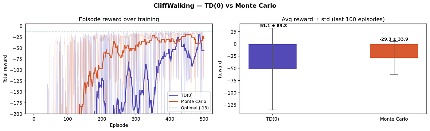
reward_curves.png shows two things side by side.

The left chart plots episode reward over training for both agents — raw (faded) and smoothed. You can see TD’s reward curve is far noisier early in training. MC’s curve is smoother and converges faster to a stable range.

The right chart shows average reward and standard deviation over the last 100 episodes as a bar chart with error bars. This makes the variance difference explicit — TD has a larger error bar because it occasionally still falls off the cliff during the epsilon-greedy exploration phase.

stds = [np.std(last_td), np.std(last_mc)]
axes[1].bar(labels, means, yerr=stds, capsize=8)

The variance difference comes from bootstrapping. TD updates based on an estimate that can itself be wrong, which compounds errors early in training. MC uses actual returns, which are noisy per episode but unbiased — the estimate is always correct for the episode that was actually played.

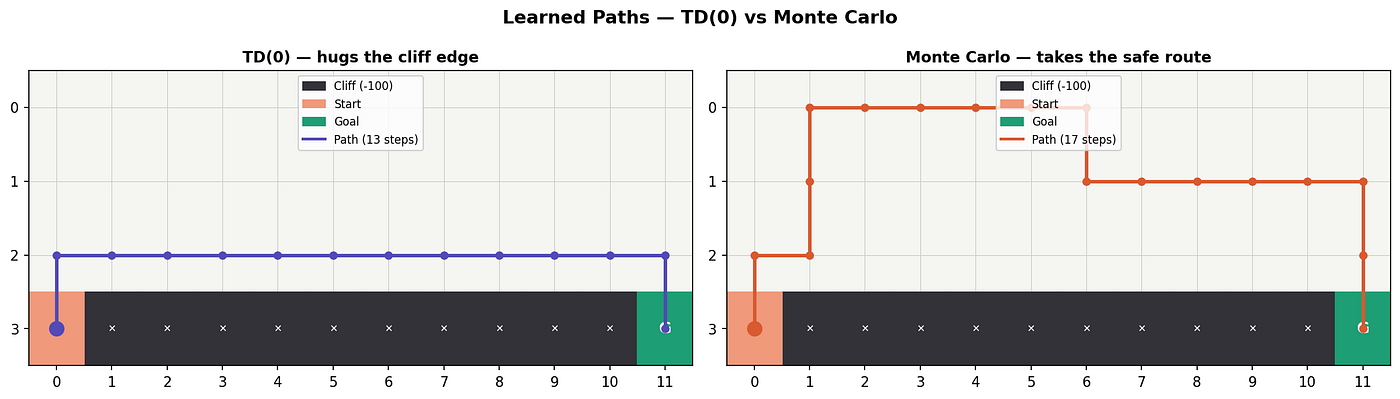
Plot 2 — Learned Paths

paths.png is the most visually striking result from this project and the one most worth putting in your article.

After training, I extract the greedy policy from each Q-table and follow it from start to goal:

def get_greedy_path(Q, env, max_steps=100):
    obs, _ = env.reset()
    path = []
    done = False
    while not done:
        row, col = divmod(obs, 12)
        path.append((row, col))
        action = int(np.argmax(Q[obs]))
        obs, _, terminated, truncated, _ = env.step(action)
        done = terminated or truncated
    return path

The resulting paths are dramatically different:

TD(0) walks along the cliff edge. It learns that the cliff cells are dangerous, but during training with epsilon-greedy it still falls in occasionally and receives the -100 penalty. Over many updates, it learns that the row directly above the cliff has slightly lower value — so it walks there anyway, because it is the shortest route and TD's bootstrapping smooths out the penalty signal across nearby states.

Monte Carlo takes the safe upper route. Because MC updates use the actual return of the full episode, a single cliff-fall gives an unambiguous -100 signal all the way back to the states that led to it. This makes those bottom-row states clearly bad, pushing the learned policy one row higher.

This is the key behavioral difference — TD is optimistic about risky states because it bootstraps away the worst outcomes. MC is pessimistic because it has actually experienced those outcomes.

Plot 3 — Value Function Heatmaps

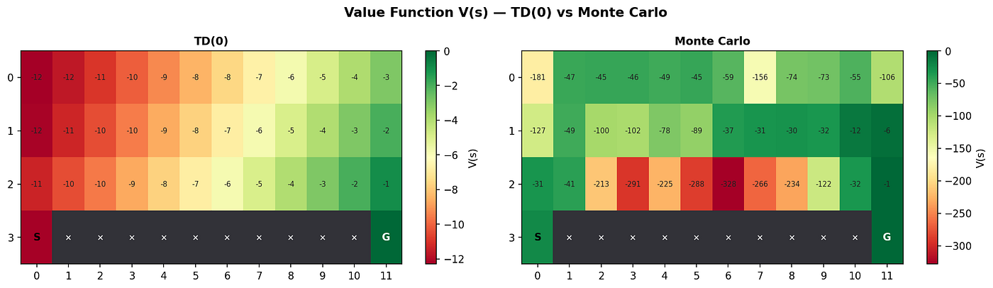
value_heatmaps.png shows V(s) = max_a Q(s,a) across the grid for both agents.

V = np.max(agent.Q, axis=1).reshape(4, 12)
ax.imshow(V, cmap='RdYlGn')

In the TD heatmap, states adjacent to the cliff still show relatively high values — the agent thinks those states are okay because it bootstraps across the cliff penalty. In the MC heatmap, those same states show clearly lower values — MC has directly experienced the -100 return from falling, and that experience is stored accurately.

The heatmap makes the internal representation of each algorithm visible — not just what path they take, but what they believe about the world.

Key Takeaways

TD bootstraps, MC does not. This is the fundamental difference. TD uses Q(s') as a proxy for the future — fast to update, but introduces bias. MC uses real returns — unbiased, but high variance because a single bad episode can swing the estimate.

Same environment, different behavior. Both algorithms find reasonable policies, but they disagree on which states are safe. TD hugs the cliff, MC avoids it. Neither is wrong — TD’s policy has higher expected reward on the optimal path, MC’s policy has lower variance because it never risks the cliff.

The paths tell the whole story. The paths.png visualization is the most important output of this project. In one image it shows that two algorithms with identical inputs — same environment, same hyperparameters, same number of episodes — learn structurally different policies because of one design choice: when to update.

Bootstrapping is a bias-variance tradeoff. TD introduces bias (it uses estimates, not true returns) in exchange for lower variance per update. MC has zero bias but higher variance. This tradeoff appears everywhere in RL — TD(λ) and n-step returns exist precisely to navigate the spectrum between these two extremes.